Machine Learning with tidymodels
Objectives
- Compare tidymodels to caret for machine learning
- Understand the components of tidymodels
- Understand the machine learning workflow using tidymodels
Overview
The caret packages are still my preferred environment to define, train, tune, assess, and generally implement machine learning in R. However, this package is being replaced by tidymodels. Similar to the tidyverse, tidymodels is not a single package, but a set of packages that function together, follow a common philosophy, and use a similar syntax. The component packages of tidymodels bring machine learning into the tidyverse. These packages use similar syntax to other tidyverse packages. So, if you like the tidyverse, you will probably like tidymodels.
Since caret has matured and is a stable, well documented tool for machine learning in R, I plan to maintain it in the course for the time being. However, eventually, I plan to replace the caret content with tidymodels examples once this environment has matured. As a transition, I am including this module to provide an introduction to tidymodels.
Again, similar to the tidyverse, tidymodels consists of several linked packages that use a similar philosophy and syntax. To install all packages, you can simply install tidymodels, which acts as a meta-package to install and load the other components. Here is a brief explanation of the component packages.
- parsnips: used to define models using a common syntax; makes it easier to experiment with different algorithms
- workflows: provides tools to create workflows, or the desired machine learning pipeline, including pre-processing, training, and post-processing
- yardstick: a one-stop-shop to implement a variety of assessment metrics for regression and classification problems
- tune: for hyperparameter tuning
- dials: for managing parameters and tuning grids
- rsample: tools for data splitting, partitioning, and resampling
- recipes: tools for pre-processing and data engineering
This website provides examples and tutorials along with links to the documentation for all the core packages discussed above.
To experiment with tidymodels, we will first use the same data explored in the random forest module, followed by a new example relating to forest community type classification. As in the random forest module, we will step through the process of creating a prediction to map the likelihood or probability of palustrine forested/palustrine scrub/shrub (PFO/PSS) wetland occurrence using a variety of terrain variables. The provided training.csv table contains 1,000 examples of PFO/PSS wetlands and 1,000 not PFO/PSS examples. The validation.csv file contains a separate, non-overlapping 2,000 examples equally split between PFO/PSS wetlands and not PFO/PSS wetlands. I will not replicate predicting back to spatial raster grids, as that process is the same when using tidymodels as it is when using caret and randomForest. The link at the bottom of the page provides the example data and R Markdown file used to generate this module.
Here is a brief description of all the provided variables.
- class: PFO/PSS (wet) or not (not)
- cost: Distance from water bodies weighted by slope
- crv_arc: Topographic curvature
- crv_plane: Plan curvature
- crv_pro: Profile curvature
- ctmi: Compound topographic moisture index (CTMI)
- diss_5: Terrain dissection (11 x 11 window)
- diss_10: Terrain dissection (21 x 21 window)
- diss_20: Terrain dissection (41 x 41 window)
- diss_25: Terrain dissection (51 x 51 window)
- diss_a: Terrain dissection average
- rough_5: Terrain roughness (11 x 11 window)
- rough_10: Terrain roughness (21 x 21 window)
- rough_20: Terrain roughness (41 x 41 window)
- rough_25: Terrain Roughness (51 x 51 window)
- rough_a: Terrain roughness average
- slp_d: Topographic slope in degrees
- sp_5: Slope position (11 x 11 window)
- sp_10: Slope position (21 x 21 window)
- sp_20: Slope position (41 x 41 window)
- sp_25: slope position (51 x 51 window)
- sp_a: Slope position average
The data provided in this example are a subset of the data used in this publication:
Maxwell, A.E., T.A. Warner, and M.P. Strager, 2016. Predicting palustrine wetland probability using random forest machine learning and digital elevation data-derived terrain variables, Photogrammetric Engineering & Remote Sensing, 82(6): 437-447. https://doi.org/10.1016/S0099-1112(16)82038-8. ## Example 1: Palustrine Wetland Occurrence Probabilistic Model (Binary Classification)
I begin by reading in the required packages. Here, tidymodels is used to load the component packages discussed above along with some other packages (e.g., ggplot2, purr, and dplyr).
library(tidymodels)Next, I set the working directory and load in the data tables. I do not want to use the last column as a predictor variable in the model, so I drop it using the select() function from dplyr.
train <- read.csv("tidymodels/training.csv", header=TRUE, sep=",", stringsAsFactors=TRUE)
test <- read.csv("tidymodels/training.csv", header=TRUE, sep=",", stringsAsFactors=TRUE)
train <- select(train, -23)
test <- select(test, -23)
The example below demonstrates a workflow for tuning and training the model. Here is the process:
- I define a model specification (tune_spec) using parsnips that indicates what model I will use (random forest), what hyperparameter values to use or tune (use 500 trees and tune the mtry parameter), what implementation of the model to use (random forest model as implemented with the ranger package), and the mode (“classification”).
- I then define a workflow (rf_wf) using the workflow() function from the workflows() package and specifying the model to use (tune_spec) and the formula (the class column predicted by all other variables in the table).
- In order to tune the hyperparameters, I define data folds (folds) and configure ten-fold cross validation using the rsample package. I also specify that folds should be stratified by the “class” field in order to maintain data balance between the two classes within each fold.
- I then set up the hyperparameter tuning process using tune_grid() from the tune package (tune_res) by specifying the workflow, folds, and the number of values to try (20).
Running all of these processes will result in a set of test hyperparameters for the defined model using a grid search and ten-fold cross validation.
tune_spec <-
  rand_forest(
    mtry = tune(),
    trees= 500
  ) %>%
  set_engine("ranger") %>%
  set_mode("classification")

rf_wf <- workflow() %>%
  add_model(tune_spec) %>%
  add_formula(class ~ .)

set.seed(123)
folds <- vfold_cv(train, v = 10, strata=class)

set.seed(123)
tune_res <- tune_grid(
  rf_wf,
  resamples = folds,
  grid = 20
)
Once the tuning process is executed, I write the results to a tibble using collect_metrics() from the tune package. Two metrics were calculated: overall accuracy and area under the receiver operating characteristic curve (AUC). The mean and standard deviation are provided for each hyperparameter combination tested, which are specifically obtained from the withheld fold for each of the ten model runs.
I then filter out the AUC results and plot them using ggplot2.
metSet <- tune_res %>% collect_metrics
metSet
# A tibble: 34 x 7
    mtry .metric  .estimator  mean     n std_err .config
   <int> <chr>    <chr>      <dbl> <int>   <dbl> <chr>
 1     3 accuracy binary     0.966    10 0.00293 Preprocessor1_Model01
 2     3 roc_auc  binary     0.992    10 0.00162 Preprocessor1_Model01
 3    16 accuracy binary     0.961    10 0.00221 Preprocessor1_Model02
 4    16 roc_auc  binary     0.992    10 0.00143 Preprocessor1_Model02
 5    20 accuracy binary     0.96     10 0.00197 Preprocessor1_Model03
 6    20 roc_auc  binary     0.992    10 0.00148 Preprocessor1_Model03
 7     4 accuracy binary     0.966    10 0.00245 Preprocessor1_Model04
 8     4 roc_auc  binary     0.991    10 0.00178 Preprocessor1_Model04
 9    12 accuracy binary     0.964    10 0.00211 Preprocessor1_Model05
10    12 roc_auc  binary     0.992    10 0.00161 Preprocessor1_Model05
# ... with 24 more rows
tune_res %>%
  collect_metrics() %>%
  filter(.metric == "roc_auc") %>%
  ggplot(aes(mtry, mean))+
  geom_point()+
  labs(x="mtry", y="AUC")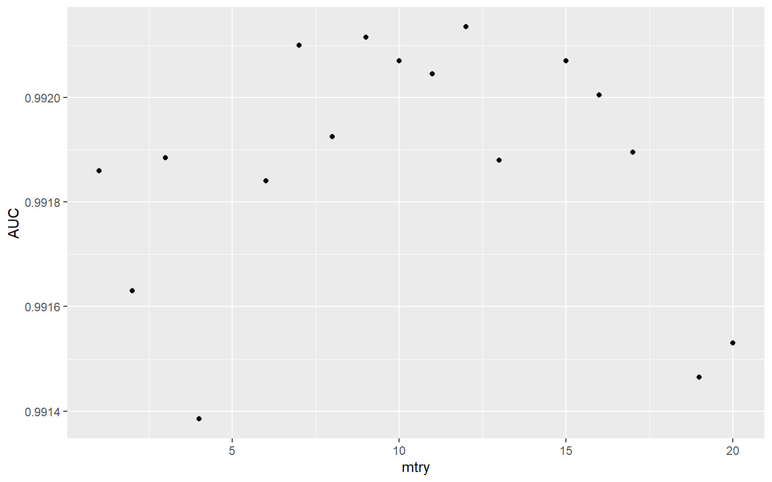
To actually obtain the best performing mtry value based on the ten-fold cross validation and the grid search tuning process, I use the select_best() function from tune and specify that I am interested in the model with the best or highest AUC.
To actually define the model with the selected mtry hyperparameter, I use the finalize_model() function from tune and specify the desired hyperparameter using the results from select_best().
best_auc <- select_best(tune_res, "roc_auc")

final_rf <- finalize_model(
  tune_spec,
  best_auc
)
Lastly, I finalize the workflow (finalize_workflow() from tune) using the finalized model and fit the model to the entire training data set.
final_wf <- rf_wf %>% finalize_workflow(final_rf)
final_fit <- final_wf %>% fit(train)
Once a trained model is obtained, it can be assessed using the withheld testing or validation set or used to predict to new data. Here, I predict the testing data set and create a new object (wet_pred) that contains the binary classification or “hard prediction”, probabilities for each class (wetland and not wetland) and the correct classification from the original testing data.
I then use the yardstick package to calculate AUC for the ROC curve using the correct classification and the predicted probability of wetland occurrence. Not that the second factor level (“wet”) is considered the positive case. Factors will be in alphabetical order unless explicitly reordered. I also calculate overall accuracy using the actual class and the predicted class.
wet_pred <- predict(final_fit, new_data = test) %>%
  bind_cols(predict(final_fit, test, type = "prob")) %>%
  bind_cols(test %>% select(class))

wet_pred %>%  roc_auc(truth = class, .pred_wet, event_level="second")
# A tibble: 1 x 3
  .metric .estimator .estimate
  <chr>   <chr>          <dbl>
1 roc_auc binary          1.00
wet_pred %>% accuracy(truth = class, .pred_class)
# A tibble: 1 x 3
  .metric  .estimator .estimate
  <chr>    <chr>          <dbl>
1 accuracy binary         0.996
Example 2: Cover Type Classification (Multiclass Classification)
In this second and new example, we will explore a multi-class classification problem using the Covertype Data Set, which I obtained from the UCI Machine Learning Repository. This data set provides a total of 581,012 instances. The goal is to differentiate seven forest community types using several environmental variables including elevation, topographic aspect, topographic slope, horizontal distance to streams, vertical distance to streams, horizontal distance to roadways, hillshade values at 9AM, hillshade values at noon, hillshade values at 3PM, horizontal distance to fire points, and a wilderness area designation, a binary and nominal variable. The seven community types are:
- 1 = Spruce/Fir
- 2 = Lodgepole Pine
- 3 = Ponderosa Pine
- 4 = Cottonwood/Willow
- 5 = Aspen
- 6 = Douglas Fir
- 7 = Krummholz
As usual, I begin by reading in the required packages and the data table. Note that a series of soil types are also included as predictor variables in the original data, but we will not use those here. Next, I use forcats to recode the numeric codes to the actual community names.
I then use dplyr to count the number of records or examples from each community type, which suggests significant data imbalance. In order to speed up the tuning and training process, I then select out 1,500 samples from each class using a stratified random sample. For potentially improved results, I should use all available samples. However, this would take a lot longer to execute. Subsetting the data is used here to speed up the example.
#Get libraries
library(tidymodels)
library(readr)
library(forcats)

#read data
coverT <- read_csv("tidymodels/covertype.csv")
coverT$cover <- as.factor(coverT$cover)
coverT$wilderness <- as.factor(coverT$wilderness)
coverT$cover <- fct_recode(coverT$cover, SpruceFir="1", LodgepolePine="2", PonderosaPine="3", CottonwoodWillow="4", Aspen="5", DouglasFir="6", Krummholz="7")
coverT %>% group_by(cover) %>% count()
# A tibble: 7 x 2
# Groups:   cover [7]
  cover                 n
  <fct>             <int>
1 SpruceFir        211840
2 LodgepolePine    283301
3 PonderosaPine     35754
4 CottonwoodWillow   2747
5 Aspen              9493
6 DouglasFir        17367
7 Krummholz         20510
#Subset data
coverT2 <- coverT %>% group_by(cover) %>% sample_n(1500)
coverT2 %>% group_by(cover) %>% count()
# A tibble: 7 x 2
# Groups:   cover [7]
  cover                n
  <fct>            <int>
1 SpruceFir         1500
2 LodgepolePine     1500
3 PonderosaPine     1500
4 CottonwoodWillow  1500
5 Aspen             1500
6 DouglasFir        1500
7 Krummholz         1500
Next, I use the parsnips package to define a random forest implementation using the “ranger” engine in “classification” mode. Note the use of tune() to indicate that I plan to tune the mtry parameter. Since the data have not already been split into separate training and testing sets, I use the initial_split() function from rsample to define training and testing partitions followed by the training() and testing() functions to create new tables for each split. Also, I am using a stratified random sample to maintain a balanced data set in both partitions.
#Define Model
rf_model <- rand_forest(mtry=tune(), trees=500) %>%
  set_engine("ranger") %>%
  set_mode("classification")

#Set split
set.seed(42)
cover_split <- initial_split(coverT2, prop=.75, strata=cover)
cover_train <- cover_split %>% training()
cover_test <- cover_split %>% testing()
I would like to normalize all continuous predictor variables and create a dummy variable from the single nominal predictor variable (“wilderness”). I define these transformations within a recipe using functions available in recipes. This also requires defining the formula and the input data. Here, I am referencing only the training set, as the test set should not be introduced to the model at this point, as this could result in a later bias assessment of model performance. The all_numeric(), all_nominal(), and all_outcomes() functions are used to select columns on which to apply the desired transformations.
The model and pre-processing recipe are then combined into a workflow.
#Define recipe
cover_recipe <- recipe(cover~., data=cover_train) %>%
  step_normalize(all_numeric()) %>%
  step_dummy(all_nominal(), -all_outcomes())

#Define workflow
cover_wf <- workflow() %>%
  add_model(rf_model) %>%
  add_recipe(cover_recipe)
I then use yardstick and the metric_set() function to define the desired assessment metrics, in this case only overall accuracy. To prepare for hyperparameter tuning using five-fold cross validation, I define folds using the vfold_cv() function from rsample. Similar to the training and testing split above, the folds are stratified by the community type to maintain class balance within each fold. Lastly, I then define values of mtry to test using the dials package. It would be better to test more values and maybe optimize additional parameters. However, I am trying to decrease the time required to execute the example.
#Define metrics
my_mets <- metric_set(accuracy)

#Define folds
set.seed(42)
cover_folds <- vfold_cv(cover_train, v=5, strata=cover)

#Define tuning grid
rf_grid <- grid_regular(mtry(range = c(1, 12)),
                        levels = 6)
Now that the model, pre-processing steps, workflow, metrics, data partitions, and mtry values to try have been defined, I tune the model using tune_grid() from the tune package. Note that this may take several minutes. Specifically, I make sure to use the defined workflow so that the pre-processing steps defined using the recipe are used. Once completed, I collect the resulting metrics for each mtry value for each fold using collect_metrics() from tune. The summarize parameter is set to FALSE because I want to obtain all results for each fold, as opposed to aggregated results. I then calculate the minimum, maximum, and median overall accuracies for each fold using dplyr and plot the results using ggplot2.
The best mtry parameter is defined using the select_best() function from tune. The workflow is then finalized and the model is trained using last_fit() from tune. The collect_predictions() function from tune is used to obtain the class prediction for each sample in the withheld test set.
rf_tuning <- cover_wf %>% tune_grid(resamples=cover_folds, grid = rf_grid, metrics=my_mets)

tune_result <- rf_tuning %>% collect_metrics(summarize=FALSE) %>%
  filter(.metric == 'accuracy') %>%
  group_by(mtry) %>%
  summarize(min_acc = min(.estimate),
            median_acc = median(.estimate),
            max_acc = max(.estimate))

ggplot(tune_result, aes(y=median_acc, x=mtry))+
  geom_point()+
  geom_errorbar(aes(ymin=min_acc, ymax=max_acc))+
  theme_bw()+
  labs(x="mtry Parameter", y = "Accuracy")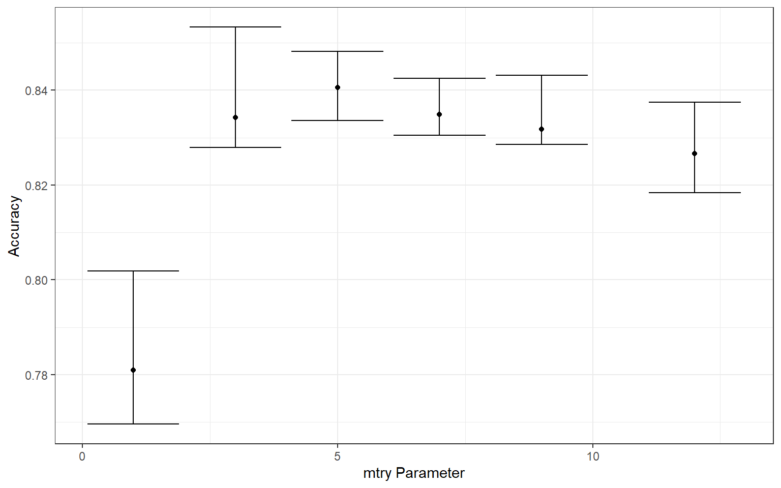
best_rf_model <- rf_tuning %>% select_best(metric="accuracy")

final_cover_wf <- cover_wf %>% finalize_workflow(best_rf_model)

final_cover_fit <- final_cover_wf %>%
  last_fit(split=cover_split, metrics=my_mets) %>% collect_predictions()
Lastly, I use the conf_mat() function from the yardstick package to obtain a multi-class error matrix from the reference and predicted classes for each sample in the withheld testing set. Passing the matrix to summmary() will provide a set of assessment metrics calculated from the error matrix.
final_cover_fit %>% conf_mat(truth=cover, estimate=.pred_class)
                  Truth
Prediction         SpruceFir LodgepolePine PonderosaPine CottonwoodWillow Aspen
  SpruceFir              284            81             0                0     1
  LodgepolePine           56           243             0                0     7
  PonderosaPine            0             9           314                8     5
  CottonwoodWillow         0             0            17              360     0
  Aspen                    7            21             4                0   358
  DouglasFir               0            16            40                7     4
  Krummholz               28             5             0                0     0
                  Truth
Prediction         DouglasFir Krummholz
  SpruceFir                 0         6
  LodgepolePine             2         2
  PonderosaPine            42         0
  CottonwoodWillow         10         0
  Aspen                     4         1
  DouglasFir              317         0
  Krummholz                 0       366
final_cover_fit %>% conf_mat(truth=cover, estimate=.pred_class) %>% summary()
# A tibble: 13 x 3
   .metric              .estimator .estimate
   <chr>                <chr>          <dbl>
 1 accuracy             multiclass     0.854
 2 kap                  multiclass     0.830
 3 sens                 macro          0.854
 4 spec                 macro          0.976
 5 ppv                  macro          0.851
 6 npv                  macro          0.976
 7 mcc                  multiclass     0.830
 8 j_index              macro          0.830
 9 bal_accuracy         macro          0.915
10 detection_prevalence macro          0.143
11 precision            macro          0.851
12 recall               macro          0.854
13 f_meas               macro          0.851
Concluding Remarks
Similar to the tidyverse, tidymodels is a very powerful framework for creating machine learning workflows and experimental environments using a common philosophy and syntax. I am still focusing on caret in this course since it is more established; however, it is planned for tidymodels to replace caret.
Although this introduction was brief and there are many more components that could be discussed, this can serve as a starting point for continued learning and experimentation. Check out the tidymodels website for additional examples and tutorials. For comparing or experimenting with multiple algorithms, I recommend checking out the workflowsets package.