Regression Techniques
Objectives
- Create linear regression models to predict a continuous variable with another continuous variable
- Use multiple linear regression to predict a continuous variable with more than one predictor variable
- Assess regression results with root mean square error (RMSE) and R-squared
- Perform regression diagnostics to assess whether assumptions are met
- Assess global spatial autocorrelation using Moran’s I
- Generate predictions using geographically weighted regression (GWR)
Overview
Before we investigate machine learning methods, this module will provide some examples of linear regression techniques to predict a continuous variable. Similar to machine learning, linear regression equations are generated by fitting to training samples. Once the model is generated, it can then be used to predict new samples. If more than one independent variable is used to predict the dependent variable, this is known as multiple regression. Since regression techniques are parametric and have assumptions, you will also need to perform diagnostics to make sure that assumptions are not violated. If data occur over a geographic extent, patterns and relationships may change over space due to spatial heterogeneity. Since the patterns are not consistent, it would not be appropriate to use a single model or equation to predict across the entire spatial extent. Instead, it would be better if the coefficients and model could change over space. Geographically weighted regression (GWR) allows for varying models across space. We will explore this technique at the end of the module.
Regression techniques are heavily used for data analysis; thus, this is a broad topic, which we will not cover in detail. For example, it is possible to use regression to predict categories or probabilities using logistic regression. It is possible to incorporate categorical predictor variables as dummy variables, model non-linear relationships with higher order terms and polynomials, and incorporate interactions. Regression techniques are also used for statistical inference; for example, ANOVA is based on regression. If you have an interest in learning more about regression, there are a variety of resources on this topic. Also, the syntax demonstrated here can be adapted to more complex techniques.
Quick-R provides examples of regression techniques here and regression diagnostics here.
In this example, we will attempt to predict the percentage of a county population that has earned at least a bachelor’s degree using other continuous variables. I obtained these data from the United States Census as estimated data as opposed to survey results. Here is a description of the provided variables. The link at the bottom of the page provides the example data and R Markdown file used to generate this module.
- per_no_hus: percent of households with no father present
- per_with_child_u18: percent of households with at least one child younger than 18
- avg_fam_size: average size of families
- percent_fem_div_15: percent of females over 15 years old that are divorced
- per_25_bach: percent of population over 25 years old with at least a bachelor’s degree
- per_native_born: percent of population born in United States
- per_eng_only: percent of population that only speaks English
- per_broadband: percent of households with broadband access
Preparation
Before beginning the analysis, you will need to read in the required packages and data. In order to join the table to the county boundaries, I create a new field from the “GEOID” field that will be unique to each county and the same as the “Unique” code provided in the Census data table.
library(ggplot2)
library(GGally)
library(tmap)
library(dplyr)
library(sf)
library(Metrics)
library(car)
library(gvlma)
library(spdep)
library(spgwr)
counties <- st_read("regression/us_counties_contig.shp")
counties$Unique <- paste0("x", as.factor(counties$GEOID))
census <- read.csv("regression/census_data.csv")I have provided the Census data as a CSV file with no associated spatial information; however, I would like to display the data in map space, so I will join it to the provided county boundaries. This is accomplished using techniques that we have already discussed. Using dplyr and the left_join() function, I join the data using the common “Unique” field.
Once the data have been joined, I use tmap to visualize the percent of the population with at least a bachelor’s degree.
data <- counties %>% left_join(census, by="Unique")tm_shape(data)+
tm_polygons(col= "per_25_bach")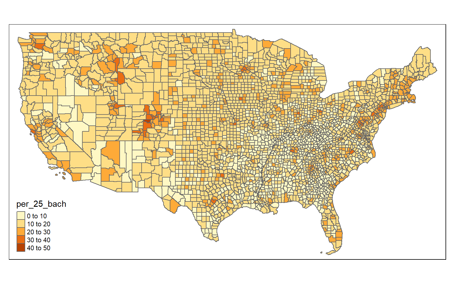
Linear Regression
Before I attempt to predict the percent of the county population with at least a bachelor’s degree with all the other provided variables, I will make a prediction using only the percent with broadband access. To visualize the relationship, I first generate a scatter plot using ggplot2. Although not perfect, it does appear that there is a relationship between these two variables. Or, higher percent access to broadband seems to be correlated with secondary degree attainment rate. This could be completely coincidental; correlation is not causation.
ggplot(data, aes(x=per_broadband, y=per_25_bach))+
geom_point()+
geom_smooth(method="lm", col="red")+
ggtitle("Broadband Access vs. Perecent of Population with at Least a Bachelor's Degree")+
labs(x="% with Broadband", y="% with At Least Bachelor's Degree")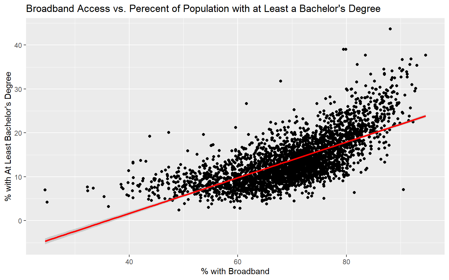
Fitting a linear model in R can be accomplished with the base R lm() function. Here, I am providing a formula. The left-side of the formula will contain the dependent variable, or the variable being predicted, while the right-side will reference one or more predictor variables. You also need to provide a data argument.
Calling summary() on the linear model will print a summary of the results. The fitted model is as follows:
per_25_bach = -14.6 + 0.41*per_broadband
Since the coefficient for the percent broadband variable is positive, this suggests that there is a positive or direct relationship between the two variables, as previously suggested by the graph generated above. The residuals vary from -15.1% to 22.5% with a median of -0.4%. The F-statistic is statistically significant, which suggest that this model is performing better than simply returning the mean value of the data set as the prediction. The R-squared value is 0.50, suggesting that roughly 50% of the variability in percent secondary degree attainment is explained by percent broadband access. In short, there is some correlation between the variables but not enough to make a strong prediction.
m1 <- lm(per_25_bach ~ per_broadband, data=data)
summary(m1)

Call:
lm(formula = per_25_bach ~ per_broadband, data = data)

Residuals:
    Min      1Q  Median      3Q     Max
-15.084  -2.760  -0.435   2.280  22.492

Coefficients:
                Estimate Std. Error t value Pr(>|t|)
(Intercept)   -14.613645   0.515371  -28.36   <2e-16 ***
per_broadband   0.406604   0.007306   55.65   <2e-16 ***
---
Signif. codes:  0 '***' 0.001 '**' 0.01 '*' 0.05 '.' 0.1 ' ' 1

Residual standard error: 3.947 on 3106 degrees of freedom
Multiple R-squared:  0.4993,    Adjusted R-squared:  0.4991
F-statistic:  3097 on 1 and 3106 DF,  p-value: < 2.2e-16
Fitted models and model summaries are stored as list objects. So, you can find specific components of the model or results within the list. In the code block below, I am extracting the R-squared value from the summary list object.
summary(m1)$r.squared
[1] 0.4992736
The Metric package can be used to calculate a variety of summary statistics. In the example below, I am using it to obtain the root mean square error (RMSE) of the model. To do so, I must provide the correct values from the original data table and the predicted or fitted values from the model list object. RMSE is reported in the units of the dependent variable, in this case percent.
rmse(data$per_25_bach, m1$fitted.values)
[1] 3.945303
You can also calculate RMSE manually as demonstrated below. This will yield the same answer as the rmse() function.
sqrt(mean((data$per_25_bach - m1$fitted.values)^2))
[1] 3.945303
Multiple Linear Regression
We will now try to predict the percent of the county population with at least a bachelor’s degree using all other variables in the Census data set. First, I generate a scatter plot matrix using the car package to visualize the distribution of the variables and the correlation between pairs. Note also that the percent of grandparents who are caretakers for at least one grandchild variable read in as a factor, so I convert it to a numeric variable before using it.
data$per_gp_gc <- as.numeric(data$per_gp_gc)
scatterplotMatrix(~per_25_bach + per_no_hus + per_with_child_u18 + avg_fam_size + per_fem_div_15 + per_native_born + per_eng_only + per_broadband, data=data, main="Variable Comparison")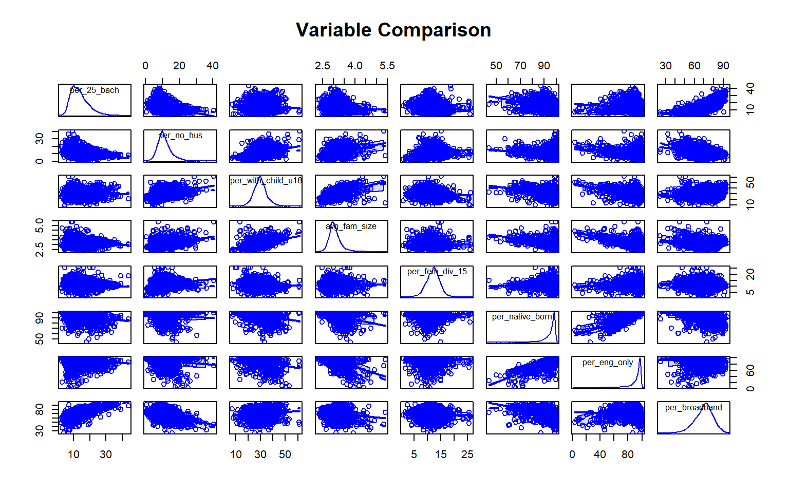
As an alternative to a scatter plot matrix, you could also just create separate scatter plots to compare the dependent variable with each independent variable separately. Take some time to analyze the patterns and correlations. What variables do you think will be most predictive?
ggplot(data, aes(x=per_no_hus, y=per_25_bach))+
geom_point()+
geom_smooth(method="lm", col="red")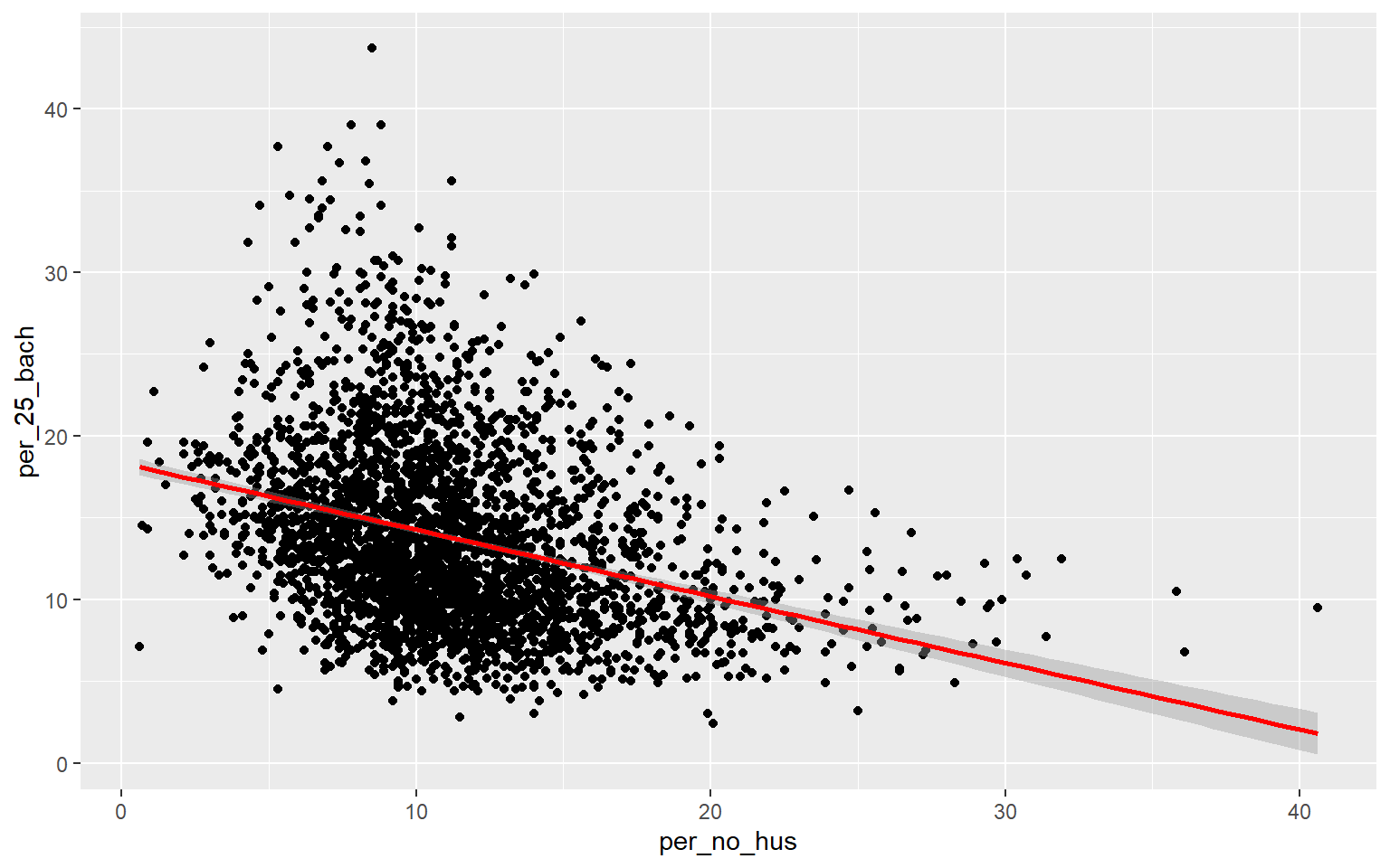
ggplot(data, aes(x=per_with_child_u18, y=per_25_bach))+
geom_point()+
geom_smooth(method="lm", col="red")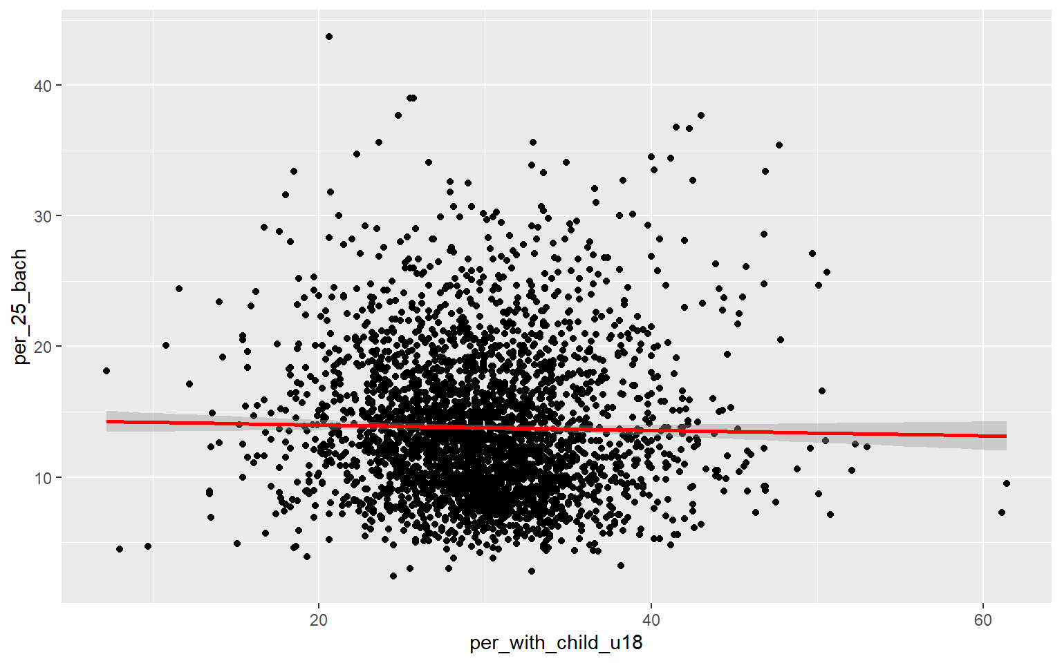
ggplot(data, aes(x=avg_fam_size, y=per_25_bach))+
geom_point()+
geom_smooth(method="lm", col="red")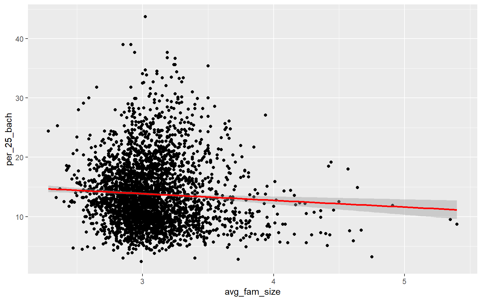
ggplot(data, aes(x=per_fem_div_15, y=per_25_bach))+
geom_point()+
geom_smooth(method="lm", col="red")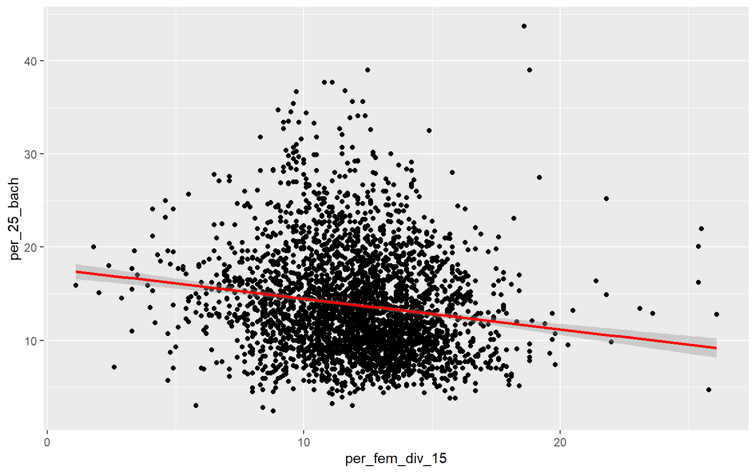
ggplot(data, aes(x=per_native_born, y=per_25_bach))+
geom_point()+
geom_smooth(method="lm", col="red")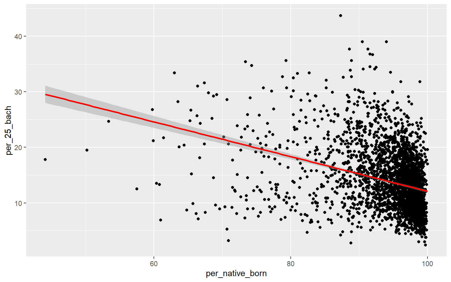
ggplot(data, aes(x=per_eng_only, y=per_25_bach))+
geom_point()+
geom_smooth(method="lm", col="red")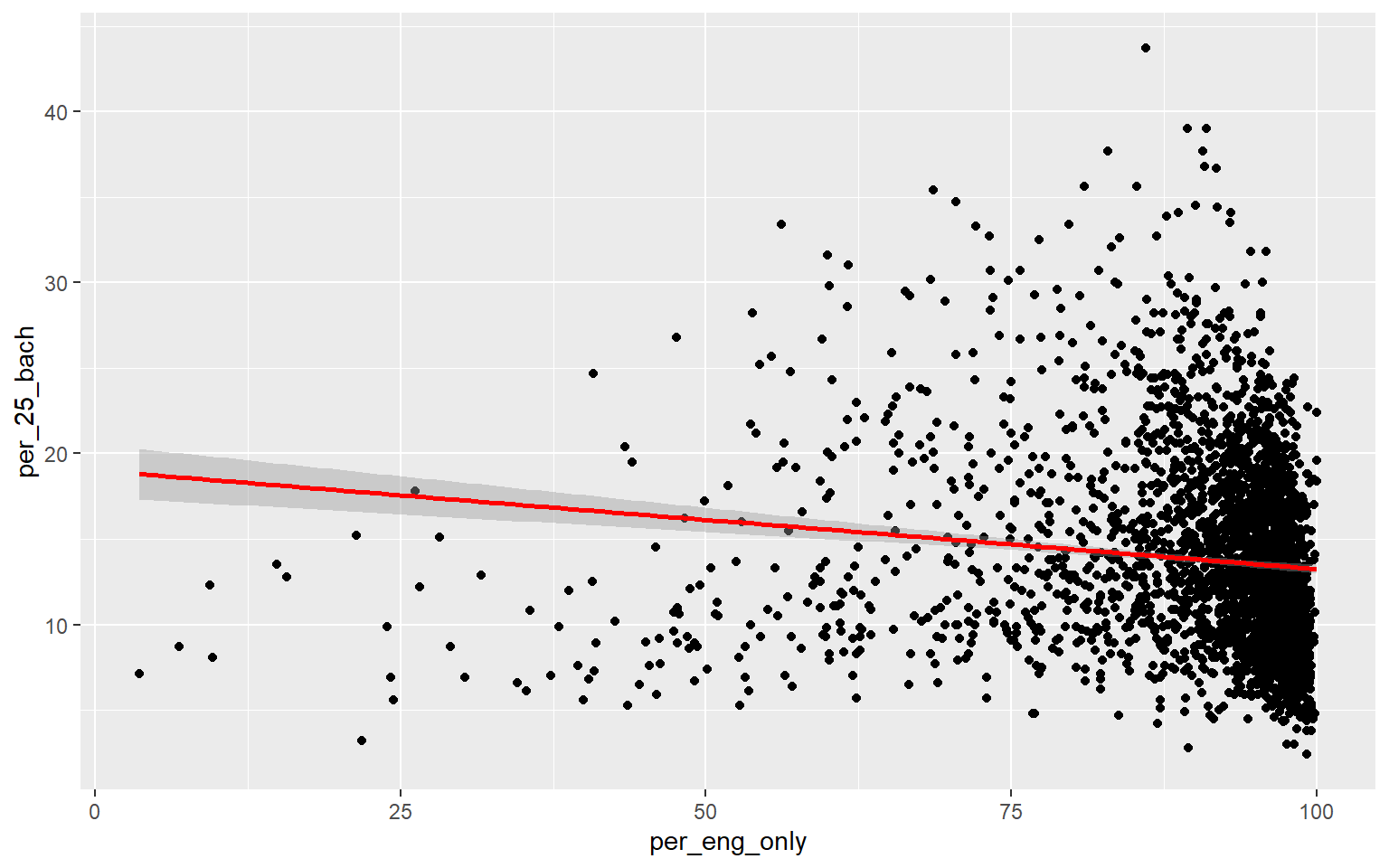
ggplot(data, aes(x=per_broadband, y=per_25_bach))+
geom_point()+
geom_smooth(method="lm", col="red")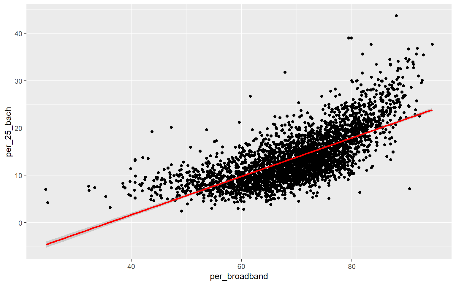
Generating a multiple linear regression model is the same as producing a linear regression model using only one independent variable accept that multiple variables will now be provided on the right-side of the equation. Once the model is generated, the summary() function can be used to explore the results. When more than one predictor variable is used, adjusted R-squared should be used for assessment as opposed to R-squared. The proportion of variance explained increased from 0.50 to 0.56, suggesting that this multiple regression model is performing better than the model created above using only percent broadband access. The F-statistic is also statistically significant, suggesting that the model is better than simply predicting using only the mean value of the dependent variable. When using multiple regression, you should interpret coefficients with caution as they don’t take into account variable correlation and can, thus, be misleading.
m2 <- lm(per_25_bach ~ per_no_hus + per_with_child_u18 + avg_fam_size + per_fem_div_15 + per_native_born + per_eng_only + per_broadband, data = data)
summary(m2)

Call:
lm(formula = per_25_bach ~ per_no_hus + per_with_child_u18 +
    avg_fam_size + per_fem_div_15 + per_native_born + per_eng_only +
    per_broadband, data = data)

Residuals:
    Min      1Q  Median      3Q     Max
-19.282  -2.421  -0.340   2.063  22.067

Coefficients:
                    Estimate Std. Error t value Pr(>|t|)
(Intercept)         4.725234   2.175156   2.172 0.029904 *
per_no_hus          0.017564   0.021002   0.836 0.403052
per_with_child_u18 -0.197942   0.015637 -12.659  < 2e-16 ***
avg_fam_size        1.742107   0.311297   5.596 2.38e-08 ***
per_fem_div_15     -0.279006   0.026547 -10.510  < 2e-16 ***
per_native_born    -0.195465   0.022383  -8.733  < 2e-16 ***
per_eng_only        0.042942   0.011772   3.648 0.000269 ***
per_broadband       0.391758   0.009277  42.228  < 2e-16 ***
---
Signif. codes:  0 '***' 0.001 '**' 0.01 '*' 0.05 '.' 0.1 ' ' 1

Residual standard error: 3.714 on 3100 degrees of freedom
Multiple R-squared:  0.5574,    Adjusted R-squared:  0.5564
F-statistic: 557.6 on 7 and 3100 DF,  p-value: < 2.2e-16
The RMSE decreased from 3.95% to 3.69%, again suggesting improvement in the model performance.
rmse(data$per_25_bach, m2$fitted.values)
[1] 3.709406
Regression Diagnostics
Once a linear regression model is produced, your work is not done. Since linear regression is a parametric method, you must test to make sure assumptions are not violated. If they are violated, you will need to correct the issue; for example, you may remove variables, transform variables, or use a different modeling method more appropriate for your data.
Here are the assumptions of linear regression:
- Residuals are normally distributed
- No patterns in the residuals relative to values of the dependent variable (homoscedasticity)
- Linear relationship exists between the dependent variable and each independent variable
- No or little multicollinearity between independent variables
- Samples are independent
Normality of the residuals can be assessed using a normal Q-Q plot. This plot can be interpreted as follows:
- On line = normal
- Concave = skewed to the right
- Convex = skewed to the left
- High/low off line = kurtosis
The code block below generates a Q-Q plot using the qqPlot() function from the car package. I have also included a simple histogram created with base R. Generally, this suggests that there may be some kurtosis issues since high and low values diverge from the line.
residuals <- data$per_25_bach - m2$fitted.values
hist(residuals)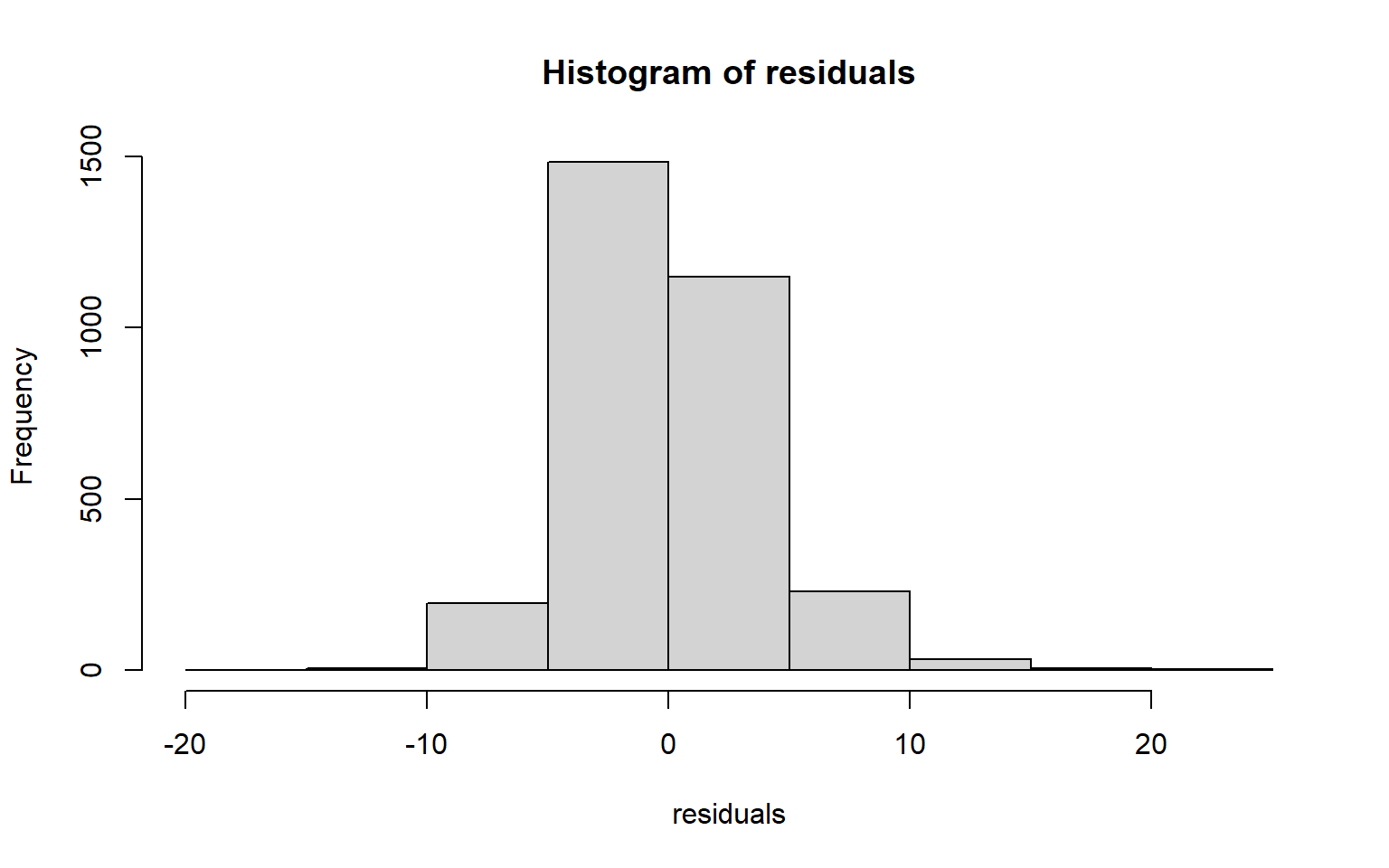
qqPlot(m2)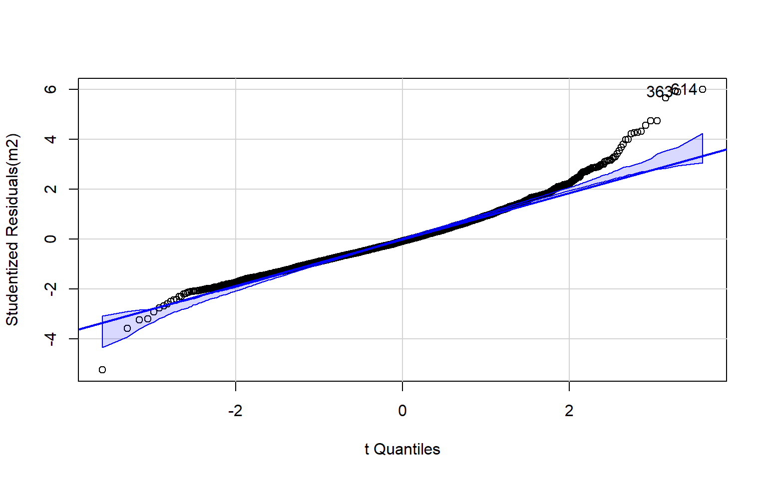
[1] 363 614Optimally, the variability in the residuals should show no pattern when plotted against the values of the dependent variable. Or, the model should not do a better or worse job at predicting high, low, or specific ranges of values of the dependent variable. This is the concept of homoscedasticity. This can be assessed using spread-level plots. In this plot, the residuals are plotted against the fitted values, and no pattern should be observed. The Score Test For Non-Constant Error Variance provides a statistical test of homoscedasticity and can be calculated in R using the ncvTest() function from the car package. In this case I obtain a statistically significant result, which suggests issues in homogeneity of variance. The test also provides a suggested power by which to transform the data.
ncvTest(m2)
Non-constant Variance Score Test
Variance formula: ~ fitted.values
Chisquare = 120.5671, Df = 1, p = < 2.22e-16
spreadLevelPlot(m2)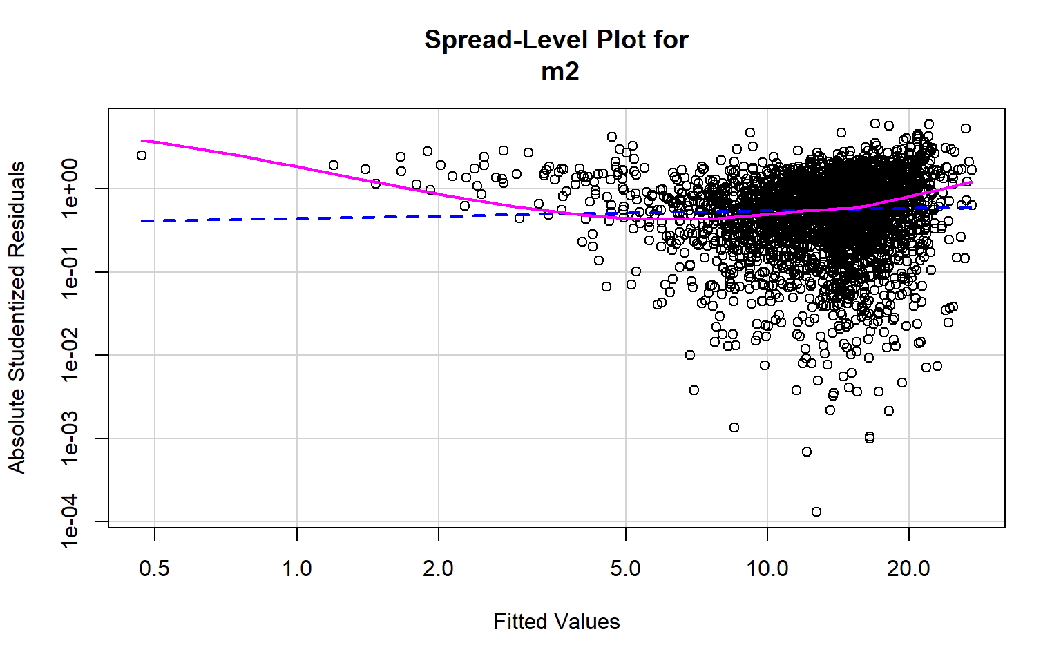
Suggested power transformation: 0.9076719 Component+Residual (Partial Residual) Plots are used to visually assess whether a linear relationship exists between the dependent variable and each independent variable. The trend should be approximated with a line. Curves and other non-linear patterns suggest that the relationship between the variables may not be linear. As an example, the relationship with percent broadband may be better modeled using a function other than a linear one. To make the relationship more linear, a data transformation could be applied.
crPlots(m2)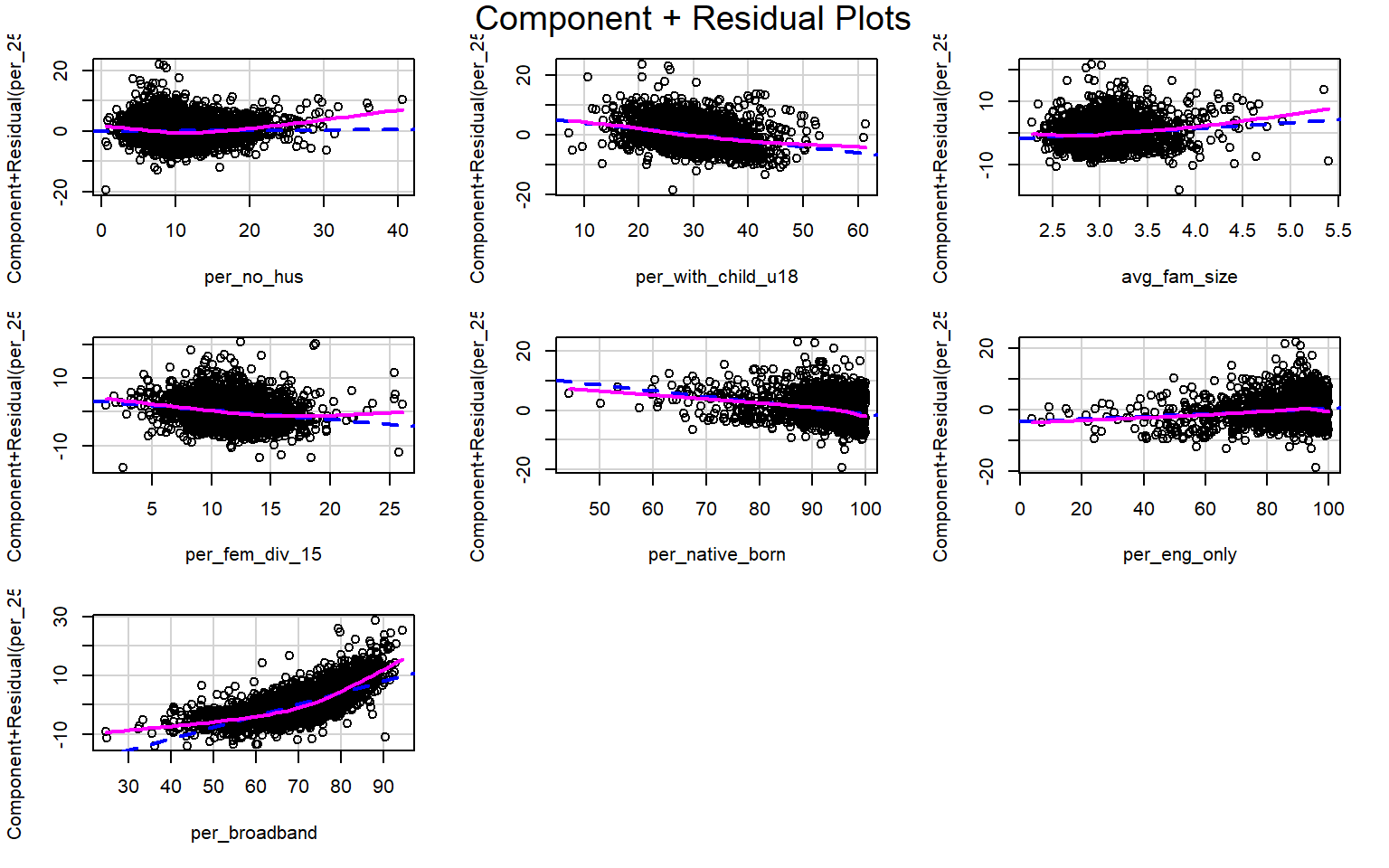
Multicollinearity between predictor variables can be assessed using the variable inflation factor (VIF). The square root of this value should not be greater than 2. This measure suggests issues with the percent native born and percent English speaking only variables. It would make sense that these variables are correlated, so it might be best to remove one of them from the model. The vif() function is provided by the car package.
vif(m2)
        per_no_hus per_with_child_u18       avg_fam_size     per_fem_div_15
          1.837697           1.736606           1.890504           1.122846
   per_native_born       per_eng_only      per_broadband
          4.128220           4.209625           1.820327
sqrt(vif(m2)) > 2 # problem?
        per_no_hus per_with_child_u18       avg_fam_size     per_fem_div_15
             FALSE              FALSE              FALSE              FALSE
   per_native_born       per_eng_only      per_broadband
              TRUE               TRUE              FALSE
The gvlma package provides the gvlma() function to test all the assumptions at once. Here are brief explanations of the components of this test.
- Global Stat: combination of all tests, if any component is not satisfied this test will not be satisfied
- Skewness: assess skewness of the residuals relative to a normal distribution
- Kurtosis: assess kurtosis of residuals relative to a normal distribution
- Link Function: assess if linear relationship exists between the dependent variable and all independent variables
- Heteroscedasticity: assess for homoscedasticity
According to this test, the only assumption that is met is homoscedasticity, which was actually found to be an issue in the test performed above. So, this regression analysis is flawed and would need to be augmented to obtain usable results. We would need to experiment with variable transformations and consider dropping some variables. If these augmentations are not successful in satisfying the assumptions, then we may need to use a method other than linear regression.
gvmodel <- gvlma(m2)
summary(gvmodel)

Call:
lm(formula = per_25_bach ~ per_no_hus + per_with_child_u18 +
    avg_fam_size + per_fem_div_15 + per_native_born + per_eng_only +
    per_broadband, data = data)

Residuals:
    Min      1Q  Median      3Q     Max
-19.282  -2.421  -0.340   2.063  22.067

Coefficients:
                    Estimate Std. Error t value Pr(>|t|)
(Intercept)         4.725234   2.175156   2.172 0.029904 *
per_no_hus          0.017564   0.021002   0.836 0.403052
per_with_child_u18 -0.197942   0.015637 -12.659  < 2e-16 ***
avg_fam_size        1.742107   0.311297   5.596 2.38e-08 ***
per_fem_div_15     -0.279006   0.026547 -10.510  < 2e-16 ***
per_native_born    -0.195465   0.022383  -8.733  < 2e-16 ***
per_eng_only        0.042942   0.011772   3.648 0.000269 ***
per_broadband       0.391758   0.009277  42.228  < 2e-16 ***
---
Signif. codes:  0 '***' 0.001 '**' 0.01 '*' 0.05 '.' 0.1 ' ' 1

Residual standard error: 3.714 on 3100 degrees of freedom
Multiple R-squared:  0.5574,    Adjusted R-squared:  0.5564
F-statistic: 557.6 on 7 and 3100 DF,  p-value: < 2.2e-16


ASSESSMENT OF THE LINEAR MODEL ASSUMPTIONS
USING THE GLOBAL TEST ON 4 DEGREES-OF-FREEDOM:
Level of Significance =  0.05

Call:
 gvlma(x = m2)

                       Value p-value                   Decision
Global Stat        1467.9292   0.000 Assumptions NOT satisfied!
Skewness            273.8103   0.000 Assumptions NOT satisfied!
Kurtosis            666.8483   0.000 Assumptions NOT satisfied!
Link Function       526.6033   0.000 Assumptions NOT satisfied!
Heteroscedasticity    0.6673   0.414    Assumptions acceptable.
Regression techniques are also generally susceptible to the impact of outliers. The outlierTest() function from the car package provides an assessment for the presence of outliers. Using this test, eight records are flagged as outliers. It might be worth experimenting with removing them from the data set to see if this improves the model and/or helps to satisfy the assumptions.
outlierTest(m2)
      rstudent unadjusted p-value Bonferroni p
614   5.984864         2.4136e-09   7.5016e-06
363   5.886481         4.3671e-09   1.3573e-05
2753  5.656594         1.6846e-08   5.2357e-05
1857 -5.252571         1.6013e-07   4.9768e-04
2203  4.735880         2.2790e-06   7.0832e-03
1624  4.724067         2.4146e-06   7.5045e-03
2703  4.544843         5.7079e-06   1.7740e-02
Leverage samples are those that have an odd or different combination of independent variable values and, thus, can have a large or disproportionate impact on the model. High leverage points can be assessed using the Cook’s Distance, as shown graphically below. Samples 499, 1042, and 1857 are identified as leverage samples that are having a large impact on the model.
cutoff <- 4/(6-length(m2$coefficients)-2)
plot(m2, which=4, cook.levels=cutoff)
abline(h=cutoff, lty=2, col="red")
Geographically Weighted Regression
Since the data used in this example occur over map space, they may not be independent or spatial heterogeneity may exist. So, it may not be appropriate to use a single equation to represent the relationships.
To determine if this is an issue, I will first plot the residuals over map space by adding the residuals to the data set then mapping them with tmap.
data$resid <- residuals
tm_shape(data)+
tm_polygons(col= "resid")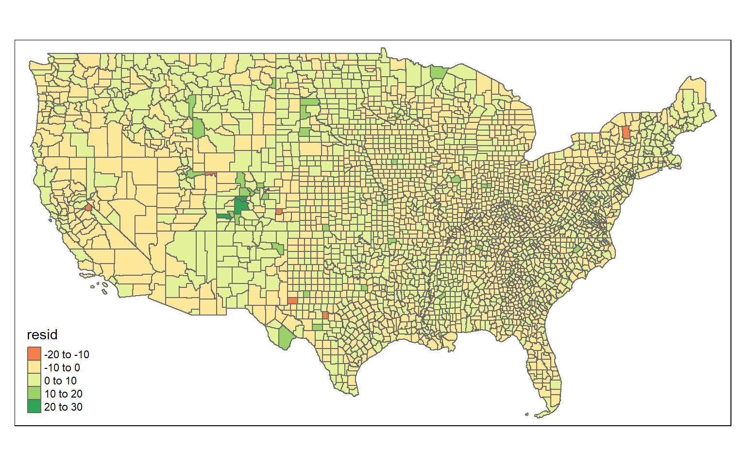
Based on a visual inspection of the map, it does appear that there may be some spatial patterns in the residuals. However, this is difficult to say with certainty. Luckily, a statistical test is available for assessing global spatial autocorrelation: Moran’s I. The null hypothesis for this test is that there is no spatial autocorrelation, or that the spatial pattern of the values is random. The alternative hypothesis is that the pattern is not random, so the values are either clustered or dispersed.
Moran’s I is based on comparing a feature to its neighbors, so we will need to obtain a matrix of weights that define spatial relationships. There are multiple means to accomplish this in R. First, I convert the sf object to an sp object, since the function of interest will not accept sf objects. Next, I build a neighbor list using the poly2nb() function from the spdep package. Using this method, only features that share boundaries will be considered neighbors. Note that there are other means to define neighbors; for example, you could use inverse distance weighting to build the spatial weights matrix. Once neighbors are defined, I use the nb2listw() function from the spdep package to build a spatial weights matrix. I can then calculate Moran’s I using the moran.test() function from spdep.
The reported Moran’s I Index is positive and statistically significant. This suggests that the residuals are spatially clustered. So, a geographically weighted regression may be more appropriate than traditional regression methods.
data_sp <- as(data, Class="Spatial")
continuity.nb <- poly2nb(data, queen = FALSE)
plot(continuity.nb, coordinates(data_sp))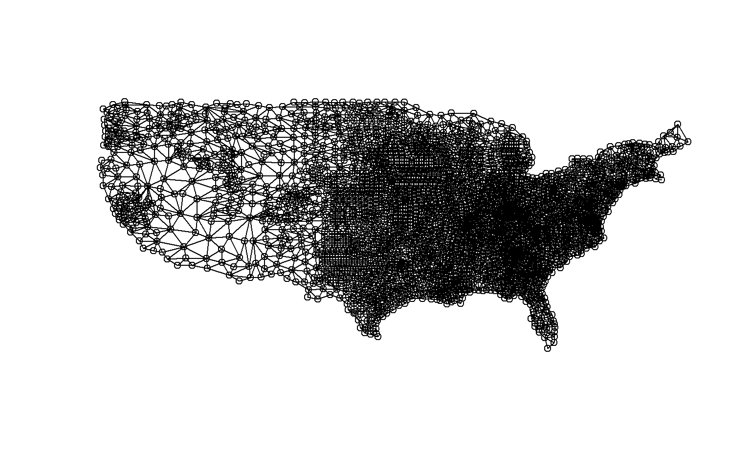
continuity.listw <- nb2listw(continuity.nb)
summary(continuity.listw)
Characteristics of weights list object:
Neighbour list object:
Number of regions: 3108
Number of nonzero links: 17752
Percentage nonzero weights: 0.1837745
Average number of links: 5.711712
Link number distribution:

   1    2    3    4    5    6    7    8    9   10   11   13
  13   26   68  341  860 1065  518  166   39   10    1    1
13 least connected regions:
294 309 367 391 680 1074 1140 1152 1498 1778 2131 2136 2351 with 1 link
1 most connected region:
1958 with 13 links

Weights style: W
Weights constants summary:
     n      nn   S0       S1       S2
W 3108 9659664 3108 1126.856 12653.89
moran.test(data_sp$resid, continuity.listw)

    Moran I test under randomisation

data:  data_sp$resid
weights: continuity.listw

Moran I statistic standard deviate = 28.746, p-value < 2.2e-16
alternative hypothesis: greater
sample estimates:
Moran I statistic       Expectation          Variance
     0.3097570180     -0.0003218539      0.0001163562
I will use the gwr() function from the spgwr package to perform geographically weighted regression. Before running the model, I will need to determine an optimal bandwidth, which defines the optimal search distance for incorporating spatial weights into the model. This can be accomplished with the gwr.sel() function.
gwr.sel(per_25_bach ~ per_no_hus + per_with_child_u18 + avg_fam_size + per_fem_div_15 + per_native_born + per_eng_only + per_broadband, data = data_sp)
Bandwidth: 2116.32 CV score: 42299.14
Bandwidth: 3420.859 CV score: 42777.43
Bandwidth: 1310.071 CV score: 41266
Bandwidth: 811.7811 CV score: 38974.97
Bandwidth: 503.8212 CV score: 35811.42
Bandwidth: 313.4915 CV score: 33243.13
Bandwidth: 195.8613 CV score: 31942.54
Bandwidth: 123.1619 CV score: 32824.8
Bandwidth: 209.3078 CV score: 32031.64
Bandwidth: 187.3723 CV score: 31902.1
Bandwidth: 162.8461 CV score: 31902.26
Bandwidth: 175.1307 CV score: 31874.44
Bandwidth: 175.1261 CV score: 31874.44
Bandwidth: 173.9778 CV score: 31874.27
Bandwidth: 169.7259 CV score: 31878.19
Bandwidth: 174.1568 CV score: 31874.27
Bandwidth: 174.1618 CV score: 31874.27
Bandwidth: 174.1607 CV score: 31874.27
Bandwidth: 174.1607 CV score: 31874.27
Bandwidth: 174.1606 CV score: 31874.27
Bandwidth: 174.1607 CV score: 31874.27
[1] 174.1607
Once the optimal bandwidth is determined, I can build the model. Note that this syntax is very similar to the regression techniques implemented above.
m3 <- gwr(per_25_bach ~ per_no_hus + per_with_child_u18 + avg_fam_size + per_fem_div_15 + per_native_born + per_eng_only + per_broadband, data = data_sp, bandwidth=74.1607)Once the model is built, I convert the result to an sf object. I then print the first five records to visualize the results. Note that different coefficients are now provided for each feature as opposed to a single, global equation. So, the model is able to vary over space to incorporate spatial heterogeneity.
m3_sf <- st_as_sf(m3$SDF)
head(m3_sf)
Simple feature collection with 6 features and 12 fields
Geometry type: MULTIPOLYGON
Dimension:     XY
Bounding box:  xmin: -123.7283 ymin: 33.99541 xmax: -96.45284 ymax: 46.38562
Geodetic CRS:  NAD83
      sum.w X.Intercept.  per_no_hus per_with_child_u18 avg_fam_size
1 23.484874    -27.42689 -0.01007355         0.04796200   2.74645886
2  9.307637     41.42467 -0.54700189        -0.20100656   1.21161468
3  4.632656     56.37373 -0.55172855         0.04579884  -5.53925238
4 23.169466    -23.20120  0.27697368        -0.03866505   0.03569103
5 20.190273    -23.26398  0.24553224        -0.02797311   1.19405230
6 21.218875    -47.50913  0.25352723        -0.24645586   4.25096646
  per_fem_div_15 per_native_born per_eng_only per_broadband      gwr.e     pred
1    -0.20456327     -0.53069283   0.52173922     0.5167422  4.1145516 11.58545
2    -0.27262219     -1.08551734   0.33595048     0.6875419 -0.9746631 10.07466
3     0.43301887     -0.21302443   0.01026571    -0.1028513 -0.2955396  5.99554
4    -0.18292220     -0.41329840   0.40358736     0.5654243  2.5396139 21.76039
5    -0.30517232     -0.50079063   0.55873024     0.4469563 -1.0036012 13.10360
6     0.05427012     -0.03128129   0.21055462     0.5455805  1.2245257 20.47547
    localR2                       geometry
1 0.7113341 MULTIPOLYGON (((-97.01952 4...
2 0.9485200 MULTIPOLYGON (((-123.4364 4...
3 0.9371532 MULTIPOLYGON (((-104.5674 3...
4 0.7364540 MULTIPOLYGON (((-96.91075 4...
5 0.6723835 MULTIPOLYGON (((-98.27367 4...
6 0.6910464 MULTIPOLYGON (((-97.12928 4...
Finally, I print the result then obtain an RMSE for the prediction. The RMSE using multiple regression obtained above is 3.69% while that for GWR is 2.7%. This suggests improvement in the prediction.
tm_shape(m3_sf)+
tm_polygons(col= "pred")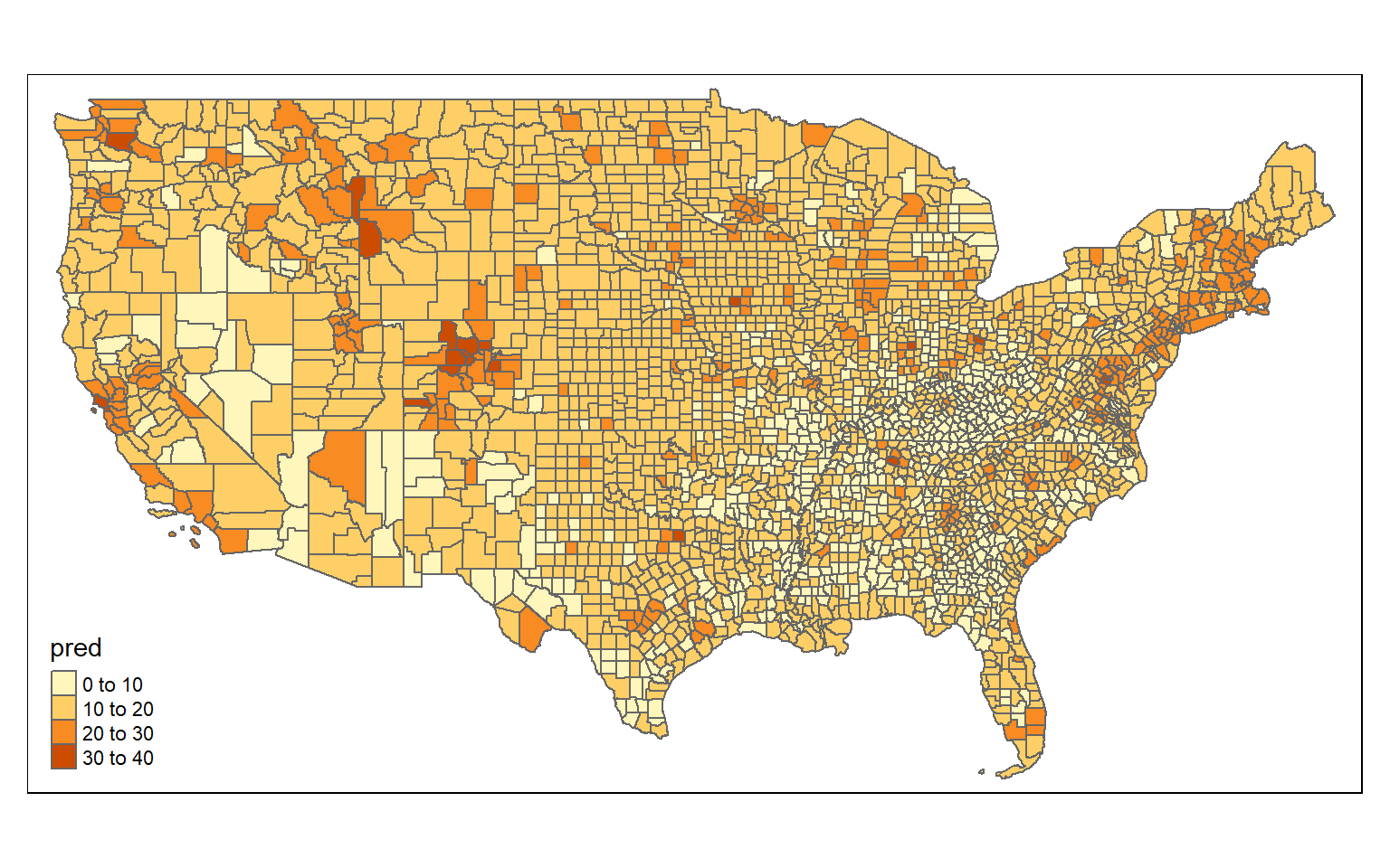
rmse(data$per_25_bach, m3_sf$pred)
[1] 1.852156
Concluding Remarks
The example used here was not optimal for linear regression as many of the model assumptions were not met. GWR improved the results; however, it also has similar assumptions that cannot be violated. So, this problem might be better tackled using a different method. We will revisit it again in the context of machine learning.