LiDAR and Image Processing in R
Objectives
- Work with large volumes of LiDAR data using LAS catalogs
- Generate raster grids from LiDAR data
- Create indices from satellite image bands
- Perform principal component analysis (PCA) and tasseled cap transformations on multispectral data
- Assess change using the difference between indices from different dates
- Apply moving windows to images
Overview
In this module I will demonstrate the processing of light detection and ranging (LiDAR) data using the lidR package. Also, this module expands upon the prior modules by demonstrating additional analyses that can be performed on raster data, specifically remotely sensed imagery. To process the image data, we will use the raster and RStoolbox packages.
In the first code block I am loading in the required packages. The link at the bottom of the page provides the example data and R Markdown file used to generate this module.
A link to the package documentation for lidR can be found here. This package is updated on a regular basis, so I recommend checking for updates periodically if you plan to use this package. Documentation for the RStoolbox package can be found here.
library(rgdal)
library(raster)
library(tmap)
library(tmaptools)
library(lidR)
library(RStoolbox)
LiDAR
Read in LiDAR Data as a LAS Catalog
Before we begin, I want to note that the LiDAR data used in the following examples are large files, as is common for point cloud data sets. So, it will take some time to execute the example code. Also, some results will be written to your hard drive. So, feel free to simply read through the examples as opposed to executing the code. The LiDAR data used in this demonstration were obtained using the WV Elevation and LiDAR Download Tool.
I have provided six adjacent tiles of LiDAR. As opposed to reading in the data separately, I will read them in as a LAS catalog, which allows you to work with and process multiple LAS files collectively. This is similar to a LAS Dataset in ArcGIS. I will focus on using LAS catalogs here with a goal of showing you how to process large volumes of LiDAR data as opposed to individual tiles. As an alternative to using LAS catalogs, you could process multiple data tiles using for loops; however, that will not be demonstrated here.
In this first example, I am reading in all six LAS files from a folder using the readLAScatalog() function. For these LiDAR data, the projection information is not read in, so I manually define the projection using the projection() function. This is not always required and depends on the LiDAR data used. The summary() function provides a summary of the data in the catalog including the spatial extent, projection, area covered, number of points (69.34 million!!!), point density, and number of files. lascheck() is used to assess if there are any issues with the data. Some issues are noted here, but they will not impact our processing and analyses. The author of the package recommends to always run this function after data are called into R to check for any issues.
las_cat <- readLAScatalog("D:/ossa/lidar")
projection(las_cat) <- "+proj=utm +zone=17 +ellps=GRS80 +datum=NAD83 +units=m +no_defs "
summary(las_cat)
class       : LAScatalog (v1.4 format 6)
extent      : 548590.2, 553090.2, 4183880, 4186880 (xmin, xmax, ymin, ymax)
coord. ref. : +proj=utm +zone=17 +datum=NAD83 +units=m +no_defs
area        : 13.5 km²
points      : 69.34million points
density     : 5.1 points/m²
num. files  : 6
proc. opt.  : buffer: 30 | chunk: 0
input opt.  : select: * | filter:
output opt. : in memory | w2w guaranteed | merging enabled
drivers     :
 - Raster : format = GTiff  NAflag = -999999
 - LAS : no parameter
 - Spatial : overwrite = FALSE
 - SimpleFeature : quiet = TRUE
 - DataFrame : no parameter
lascheck(las_cat)

 Checking headers consistency
  - Checking file version consistency... <U+2713>
  - Checking scale consistency... <U+2713>
  - Checking offset consistency... <U+2713>
  - Checking point type consistency... <U+2713>
  - Checking VLR consistency...
    <U+2717> Inconsistent number of VLR
  - Checking CRS consistency... <U+2713>
 Checking the headers
  - Checking scale factor validity... <U+2713>
  - Checking Point Data Format ID validity... <U+2713>
 Checking preprocessing already done
  - Checking negative outliers... <U+2713>
  - Checking normalization... no
 Checking the geometry
  - Checking overlapping tiles... <U+2713>
  - Checking point indexation... no
Create a DTM
Before starting an analysis of all data in a LAS catalog, you will need to define some processing options. In the code block below I am defining processing “chunks” as 500-by-500 meter tiles with a 20 meter overlap. It is generally good to define an overlap to avoid any gaps in generated raster grid surfaces. You will need to experiment with appropriate chunk sizes. This will depend on the point density of the data and the available memory in your computer. The goal is to provide small enough tiles so that you will not run out of memory but not too small to produce a lot of tiles and process the data inefficiently. I am also having the process write a processing summary. The processing options are stored within the LAS catalog object, as demonstrated by summarizing the object.
opt_chunk_size(las_cat) <- 500
plot(las_cat, chunk_pattern = TRUE)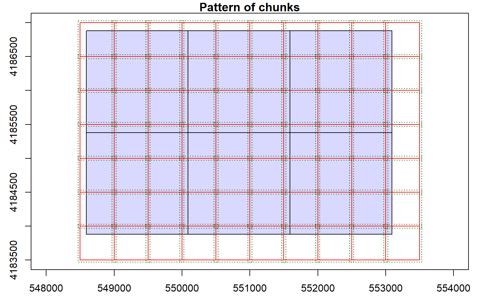
opt_chunk_buffer(las_cat) <- 20
plot(las_cat, chunk_pattern = TRUE)
summary(las_cat)
class       : LAScatalog (v1.4 format 6)
extent      : 548590.2, 553090.2, 4183880, 4186880 (xmin, xmax, ymin, ymax)
coord. ref. : +proj=utm +zone=17 +datum=NAD83 +units=m +no_defs
area        : 13.5 km²
points      : 69.34million points
density     : 5.1 points/m²
num. files  : 6
proc. opt.  : buffer: 20 | chunk: 500
input opt.  : select: * | filter:
output opt. : in memory | w2w guaranteed | merging enabled
drivers     :
 - Raster : format = GTiff  NAflag = -999999
 - LAS : no parameter
 - Spatial : overwrite = FALSE
 - SimpleFeature : quiet = TRUE
 - DataFrame : no parameter
Once processing options are defined, you can perform analyses and process the data. In this example, I am creating a digital terrain model (DTM) to represent ground elevations without any above ground features. I am also setting a new processing option to indicate where to store the resulting raster grids on the local disk. Each tile will be labeled with the bottom-left coordinate of the extent. Within the grid_terrain() function, I am setting the output cell size to 2-by-2 meters and I am using the k-nearest neighbor inverse distance weighting interpolation method with 10 neighbors and a power of 2.
opt_output_files(las_cat) <- "D:/ossa/las_out/dtm_{XLEFT}_{YBOTTOM}"
dtm <- grid_terrain(las_cat, res = 2, knnidw(k = 10, p = 2), keep_lowest = FALSE)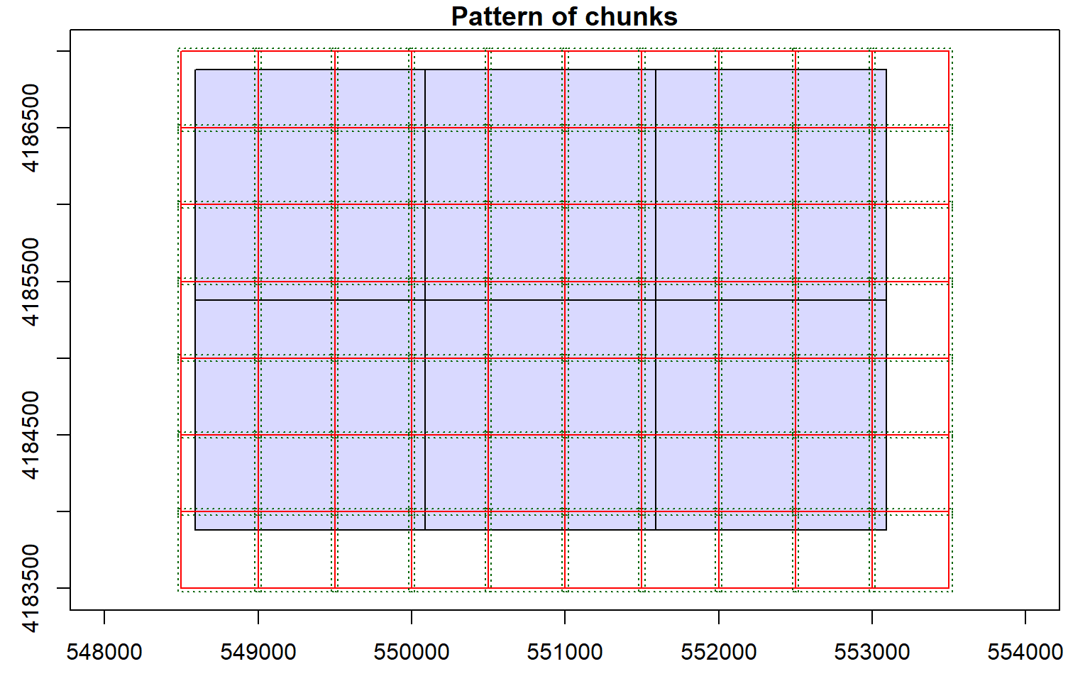
Chunk 1 of 70 (1.4%): state <U+26A0>
Chunk 2 of 70 (2.9%): state <U+26A0>
Chunk 3 of 70 (4.3%): state <U+26A0>
Chunk 4 of 70 (5.7%): state <U+26A0>
Chunk 5 of 70 (7.1%): state <U+26A0>
Chunk 6 of 70 (8.6%): state <U+26A0>
Chunk 7 of 70 (10%): state <U+26A0>
Chunk 8 of 70 (11.4%): state <U+26A0>
Chunk 9 of 70 (12.9%): state <U+26A0>
Chunk 10 of 70 (14.3%): state <U+2713>
Chunk 11 of 70 (15.7%): state <U+26A0>
Chunk 12 of 70 (17.1%): state <U+26A0>
Chunk 13 of 70 (18.6%): state <U+26A0>
Chunk 14 of 70 (20%): state <U+26A0>
Chunk 15 of 70 (21.4%): state <U+26A0>
Chunk 16 of 70 (22.9%): state <U+26A0>
Chunk 17 of 70 (24.3%): state <U+26A0>
Chunk 18 of 70 (25.7%): state <U+26A0>
Chunk 19 of 70 (27.1%): state <U+26A0>
Chunk 20 of 70 (28.6%): state <U+26A0>
Chunk 21 of 70 (30%): state <U+26A0>
Chunk 22 of 70 (31.4%): state <U+26A0>
Chunk 23 of 70 (32.9%): state <U+26A0>
Chunk 24 of 70 (34.3%): state <U+26A0>
Chunk 25 of 70 (35.7%): state <U+26A0>
Chunk 26 of 70 (37.1%): state <U+26A0>
Chunk 27 of 70 (38.6%): state <U+26A0>
Chunk 28 of 70 (40%): state <U+26A0>
Chunk 29 of 70 (41.4%): state <U+26A0>
Chunk 30 of 70 (42.9%): state <U+26A0>
Chunk 31 of 70 (44.3%): state <U+26A0>
Chunk 32 of 70 (45.7%): state <U+26A0>
Chunk 33 of 70 (47.1%): state <U+26A0>
Chunk 34 of 70 (48.6%): state <U+26A0>
Chunk 35 of 70 (50%): state <U+26A0>
Chunk 36 of 70 (51.4%): state <U+26A0>
Chunk 37 of 70 (52.9%): state <U+26A0>
Chunk 38 of 70 (54.3%): state <U+26A0>
Chunk 39 of 70 (55.7%): state <U+26A0>
Chunk 40 of 70 (57.1%): state <U+26A0>
Chunk 41 of 70 (58.6%): state <U+26A0>
Chunk 42 of 70 (60%): state <U+26A0>
Chunk 43 of 70 (61.4%): state <U+26A0>
Chunk 44 of 70 (62.9%): state <U+26A0>
Chunk 45 of 70 (64.3%): state <U+26A0>
Chunk 46 of 70 (65.7%): state <U+26A0>
Chunk 47 of 70 (67.1%): state <U+26A0>
Chunk 48 of 70 (68.6%): state <U+26A0>
Chunk 49 of 70 (70%): state <U+26A0>
Chunk 50 of 70 (71.4%): state <U+26A0>
Chunk 51 of 70 (72.9%): state <U+26A0>
Chunk 52 of 70 (74.3%): state <U+26A0>
Chunk 53 of 70 (75.7%): state <U+26A0>
Chunk 54 of 70 (77.1%): state <U+26A0>
Chunk 55 of 70 (78.6%): state <U+26A0>
Chunk 56 of 70 (80%): state <U+26A0>
Chunk 57 of 70 (81.4%): state <U+26A0>
Chunk 58 of 70 (82.9%): state <U+26A0>
Chunk 59 of 70 (84.3%): state <U+26A0>
Chunk 60 of 70 (85.7%): state <U+26A0>
Chunk 61 of 70 (87.1%): state <U+26A0>
Chunk 62 of 70 (88.6%): state <U+26A0>
Chunk 63 of 70 (90%): state <U+26A0>
Chunk 64 of 70 (91.4%): state <U+26A0>
Chunk 65 of 70 (92.9%): state <U+26A0>
Chunk 66 of 70 (94.3%): state <U+26A0>
Chunk 67 of 70 (95.7%): state <U+26A0>
Chunk 68 of 70 (97.1%): state <U+26A0>
Chunk 69 of 70 (98.6%): state <U+26A0>
Chunk 70 of 70 (100%): state <U+26A0>
Once the results are generated, the individual tiles will be stored on disk but also referenced to a virtual raster mosaic object for additional processing. Note that it is possible to store the raster data in memory, but this is not recommended if you are processing a large volume of data.
As already suggested, it is generally a good idea to visualize the result. Below I am using tmap to visualize the terrain model.
tm_shape(dtm)+
tm_raster(style= "quantile", palette=get_brewer_pal("Greys", plot=FALSE))+
tm_layout(legend.outside = TRUE)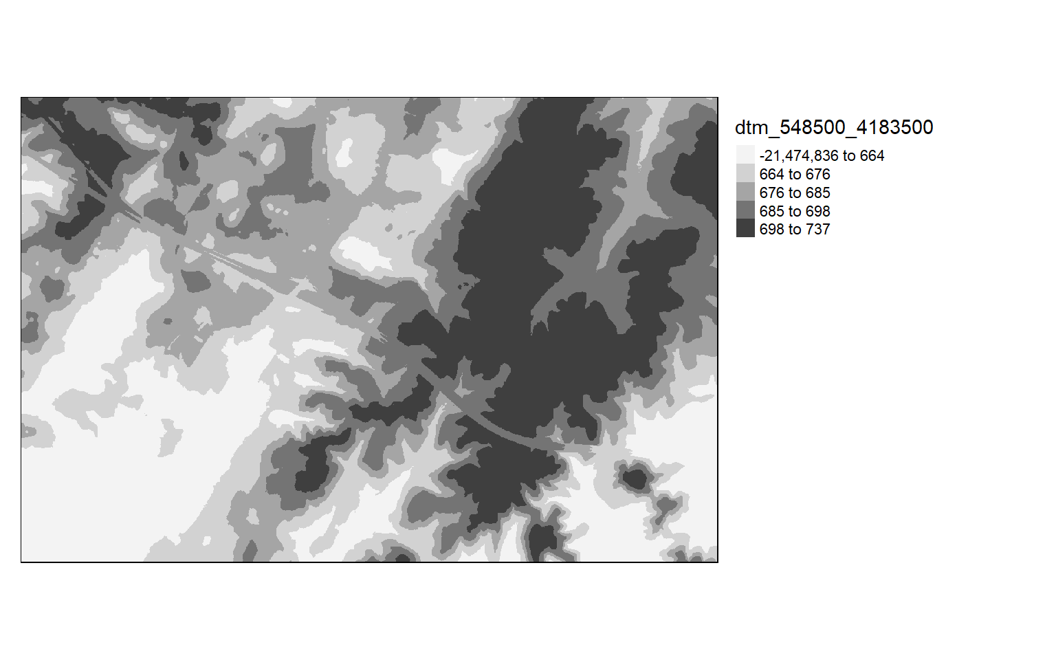
You can write the produced virtual raster mosaic to disk as a single continuous grid using the writeRaster() function from the raster package. It is not advisable to do so if a large volume of data is processed and/or the cell size is small, as the file may be extremely large.
writeRaster(dtm, "D:/ossa/las_out/dtm.tif")Create a Hillshade
A hillshade offers a means to visualize a terrain surface by modeling illumination over the terrain using a defined illuminating position. The process of producing a hillshade in R is different from the process in ArcGIS. First, you will need to produce slope and aspect surfaces. You will then use these surfaces to generate the hillshade with a defined illuminating position. All the required functions are made available by the raster package. In the example, the illuminating source has been placed at a northwestern position and at an angle of 45-degrees above the horizon. In the next block of code the hillshade is displayed using tmap.
slope <- terrain(dtm, opt='slope')
aspect <- terrain(dtm, opt='aspect')
hs <- hillShade(slope, aspect, angle=45, direction=315)tm_shape(hs)+
tm_raster(style= "cont", palette=get_brewer_pal("Greys", plot=FALSE))+
tm_layout(legend.outside = TRUE)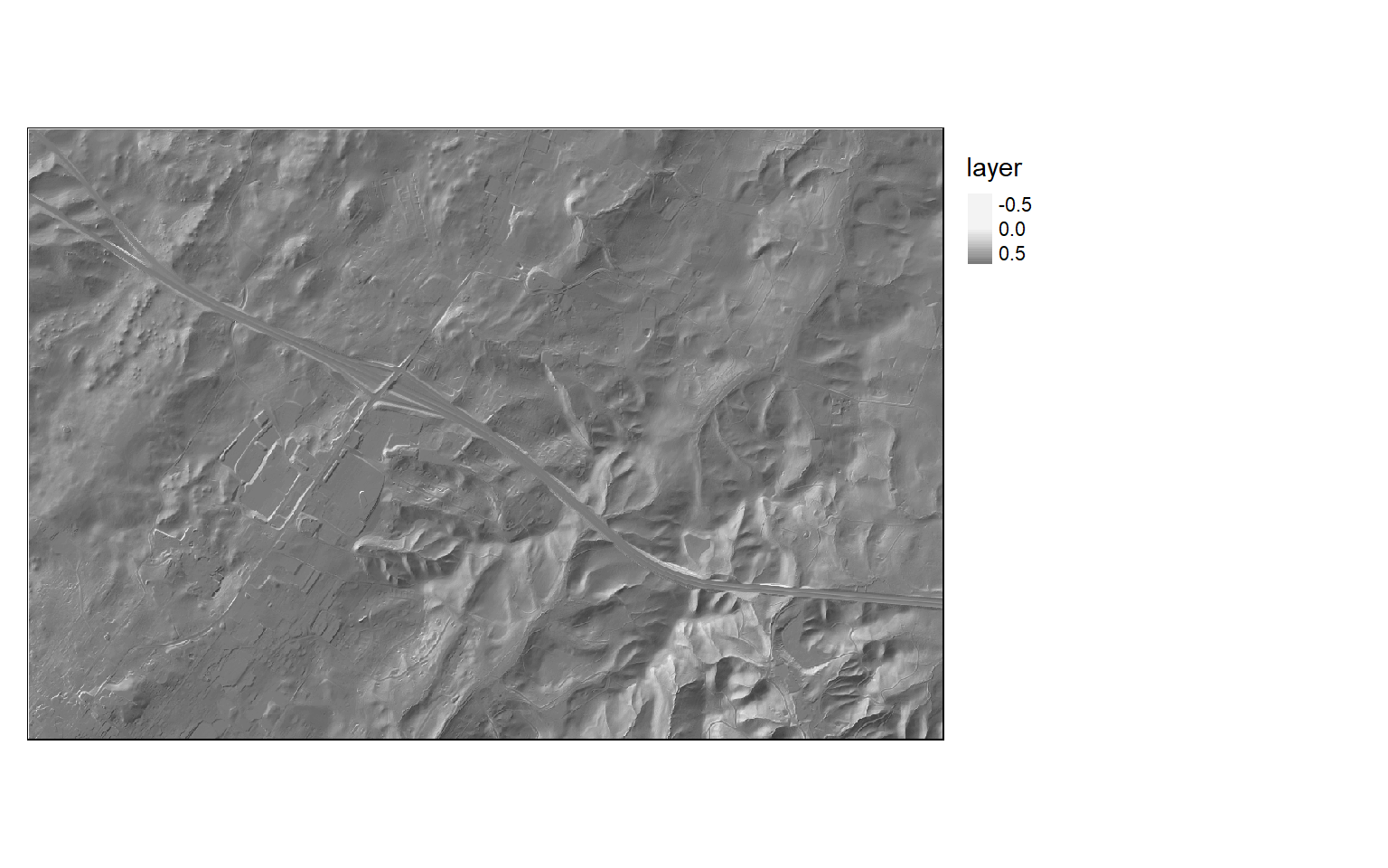
Create a nDSM
The lasnormalize() function is used to subtract ground elevations from each point and requires input LAS data and a DTM. The result is LAS files written to disk. Here, I have provided a new folder path in which to store the output. Once these points are generated, they can be used to produce a canopy height model (CHM) or normalized digital surface model (nDSM) where the grid values represent heights of features above the ground.
opt_output_files(las_cat) <- "D:/ossa/las_out/norm/norm_{XLEFT}_{YBOTTOM}"
lasnorm <- normalize_height(las_cat, dtm)
The grid_canopy() function is used to generate a digital surface model (DSM). If normalized data are provided, the result will be a CHM or nDSM. In this example, I am using the original point cloud data that have not been normalized. Once the surface is produced, it can be written out to a permanent file. I am also using the pitfree algorithm to generate a smoothed model or remove pits.
opt_output_files(las_cat) <- "D:/ossa/las_out/dsm/dsm_{XLEFT}_{YBOTTOM}"
dsm <- grid_canopy(las_cat, res = 2, pitfree(c(0,2,5,10,15), c(0, 1)))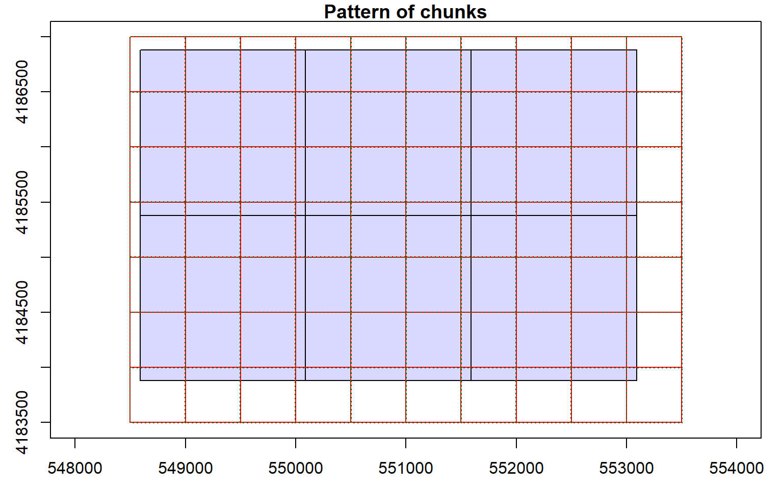
Chunk 1 of 70 (1.4%): state <U+2713>
Chunk 2 of 70 (2.9%): state <U+2713>
Chunk 3 of 70 (4.3%): state <U+2713>
Chunk 4 of 70 (5.7%): state <U+2713>
Chunk 5 of 70 (7.1%): state <U+2713>
Chunk 6 of 70 (8.6%): state <U+2713>
Chunk 7 of 70 (10%): state <U+2713>
Chunk 8 of 70 (11.4%): state <U+2713>
Chunk 9 of 70 (12.9%): state <U+2713>
Chunk 10 of 70 (14.3%): state <U+2713>
Chunk 11 of 70 (15.7%): state <U+2713>
Chunk 12 of 70 (17.1%): state <U+2713>
Chunk 13 of 70 (18.6%): state <U+2713>
Chunk 14 of 70 (20%): state <U+2713>
Chunk 15 of 70 (21.4%): state <U+2713>
Chunk 16 of 70 (22.9%): state <U+2713>
Chunk 17 of 70 (24.3%): state <U+2713>
Chunk 18 of 70 (25.7%): state <U+2713>
Chunk 19 of 70 (27.1%): state <U+2713>
Chunk 20 of 70 (28.6%): state <U+2713>
Chunk 21 of 70 (30%): state <U+2713>
Chunk 22 of 70 (31.4%): state <U+2713>
Chunk 23 of 70 (32.9%): state <U+2713>
Chunk 24 of 70 (34.3%): state <U+2713>
Chunk 25 of 70 (35.7%): state <U+2713>
Chunk 26 of 70 (37.1%): state <U+2713>
Chunk 27 of 70 (38.6%): state <U+2713>
Chunk 28 of 70 (40%): state <U+2713>
Chunk 29 of 70 (41.4%): state <U+2713>
Chunk 30 of 70 (42.9%): state <U+2713>
Chunk 31 of 70 (44.3%): state <U+2713>
Chunk 32 of 70 (45.7%): state <U+2713>
Chunk 33 of 70 (47.1%): state <U+2713>
Chunk 34 of 70 (48.6%): state <U+2713>
Chunk 35 of 70 (50%): state <U+2713>
Chunk 36 of 70 (51.4%): state <U+2713>
Chunk 37 of 70 (52.9%): state <U+2713>
Chunk 38 of 70 (54.3%): state <U+2713>
Chunk 39 of 70 (55.7%): state <U+2713>
Chunk 40 of 70 (57.1%): state <U+2713>
Chunk 41 of 70 (58.6%): state <U+2713>
Chunk 42 of 70 (60%): state <U+2713>
Chunk 43 of 70 (61.4%): state <U+2713>
Chunk 44 of 70 (62.9%): state <U+2713>
Chunk 45 of 70 (64.3%): state <U+2713>
Chunk 46 of 70 (65.7%): state <U+2713>
Chunk 47 of 70 (67.1%): state <U+2713>
Chunk 48 of 70 (68.6%): state <U+2713>
Chunk 49 of 70 (70%): state <U+2713>
Chunk 50 of 70 (71.4%): state <U+2713>
Chunk 51 of 70 (72.9%): state <U+2713>
Chunk 52 of 70 (74.3%): state <U+2713>
Chunk 53 of 70 (75.7%): state <U+2713>
Chunk 54 of 70 (77.1%): state <U+2713>
Chunk 55 of 70 (78.6%): state <U+2713>
Chunk 56 of 70 (80%): state <U+2713>
Chunk 57 of 70 (81.4%): state <U+2713>
Chunk 58 of 70 (82.9%): state <U+2713>
Chunk 59 of 70 (84.3%): state <U+2713>
Chunk 60 of 70 (85.7%): state <U+2713>
Chunk 61 of 70 (87.1%): state <U+2713>
Chunk 62 of 70 (88.6%): state <U+2713>
Chunk 63 of 70 (90%): state <U+2713>
Chunk 64 of 70 (91.4%): state <U+2713>
Chunk 65 of 70 (92.9%): state <U+2713>
Chunk 66 of 70 (94.3%): state <U+2713>
Chunk 67 of 70 (95.7%): state <U+2713>
Chunk 68 of 70 (97.1%): state <U+2713>
Chunk 69 of 70 (98.6%): state <U+2713>
Chunk 70 of 70 (100%): state <U+2713>writeRaster(dsm, "D:/ossa/las_out/dsm.tif")Since I used the original data that have not been normalized, in order to generate an nDSM, I subtract the DTM from the DSM. It is common to obtain some negative values due to noise in the data. So, I then convert all cells that have a negative height to zero and print the data information to inspect the result.
Again, I visualize the result with tmap.
ndsm <- dsm - dtm
ndsm[ndsm<0]=0
ndsm
class      : RasterLayer
dimensions : 1501, 2251, 3378751  (nrow, ncol, ncell)
resolution : 2, 2  (x, y)
extent     : 548590, 553092, 4183878, 4186880  (xmin, xmax, ymin, ymax)
crs        : +proj=utm +zone=17 +datum=NAD83 +units=m +no_defs
source     : memory
names      : layer
values : 0, 21475507 (min, max)tm_shape(ndsm)+
tm_raster(style= "quantile", n=7, palette=get_brewer_pal("Greens", n=7, plot=FALSE))+
tm_layout(legend.outside = TRUE)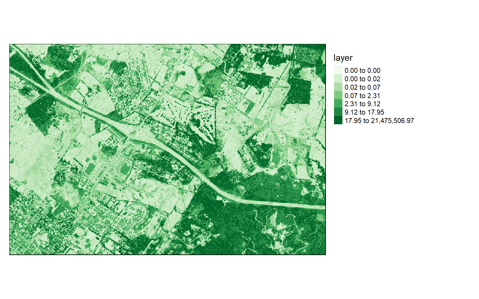
Calculate Point Cloud Statistics in Cells
It is also possible to calculate a statistic from the point data within each grid cell using the grid_metrics() function. In the example, I am calculating the mean elevation from the first return data within 10-by-10 meter cells. Before doing so, I define a filter option so that only the first returns are used. I then display the results using tmap.
opt_output_files(las_cat) <- "D:/ossa/las_out/means/means_{XLEFT}_{YBOTTOM}"
opt_filter(las_cat) <- "-keep_first"
metrics <- grid_metrics(las_cat, ~mean(Z), 10)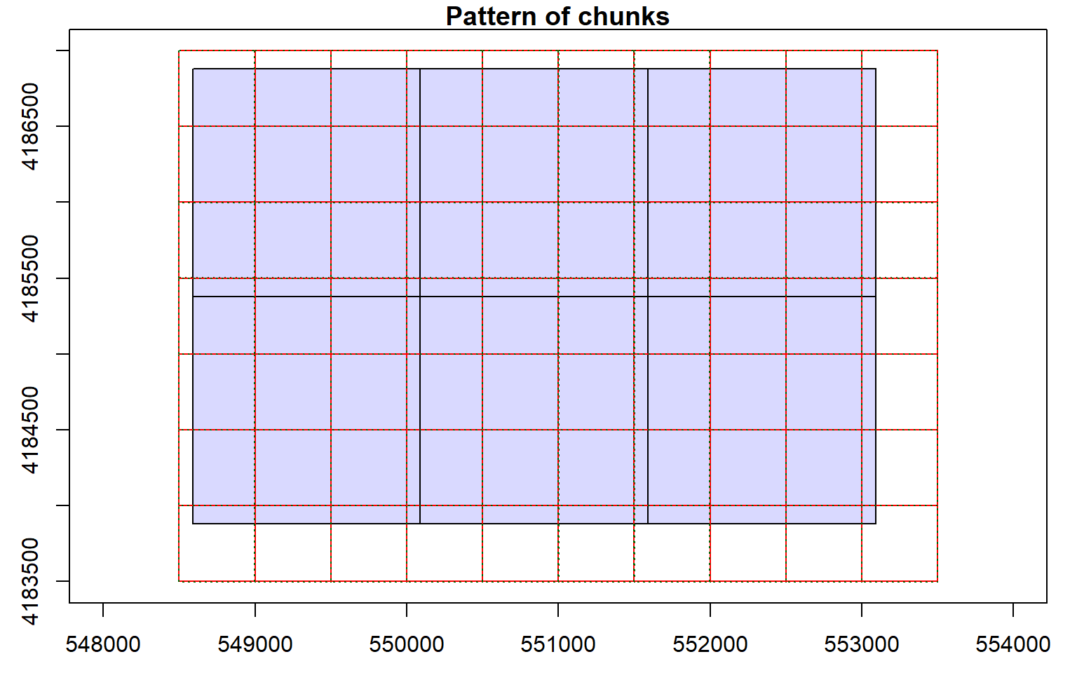
Chunk 1 of 70 (1.4%): state <U+2713>
Chunk 2 of 70 (2.9%): state <U+2713>
Chunk 3 of 70 (4.3%): state <U+2713>
Chunk 4 of 70 (5.7%): state <U+2713>
Chunk 5 of 70 (7.1%): state <U+2713>
Chunk 6 of 70 (8.6%): state <U+2713>
Chunk 7 of 70 (10%): state <U+2713>
Chunk 8 of 70 (11.4%): state <U+2713>
Chunk 9 of 70 (12.9%): state <U+2713>
Chunk 10 of 70 (14.3%): state <U+2713>
Chunk 11 of 70 (15.7%): state <U+2713>
Chunk 12 of 70 (17.1%): state <U+2713>
Chunk 13 of 70 (18.6%): state <U+2713>
Chunk 14 of 70 (20%): state <U+2713>
Chunk 15 of 70 (21.4%): state <U+2713>
Chunk 16 of 70 (22.9%): state <U+2713>
Chunk 17 of 70 (24.3%): state <U+2713>
Chunk 18 of 70 (25.7%): state <U+2713>
Chunk 19 of 70 (27.1%): state <U+2713>
Chunk 20 of 70 (28.6%): state <U+2713>
Chunk 21 of 70 (30%): state <U+2713>
Chunk 22 of 70 (31.4%): state <U+2713>
Chunk 23 of 70 (32.9%): state <U+2713>
Chunk 24 of 70 (34.3%): state <U+2713>
Chunk 25 of 70 (35.7%): state <U+2713>
Chunk 26 of 70 (37.1%): state <U+2713>
Chunk 27 of 70 (38.6%): state <U+2713>
Chunk 28 of 70 (40%): state <U+2713>
Chunk 29 of 70 (41.4%): state <U+2713>
Chunk 30 of 70 (42.9%): state <U+2713>
Chunk 31 of 70 (44.3%): state <U+2713>
Chunk 32 of 70 (45.7%): state <U+2713>
Chunk 33 of 70 (47.1%): state <U+2713>
Chunk 34 of 70 (48.6%): state <U+2713>
Chunk 35 of 70 (50%): state <U+2713>
Chunk 36 of 70 (51.4%): state <U+2713>
Chunk 37 of 70 (52.9%): state <U+2713>
Chunk 38 of 70 (54.3%): state <U+2713>
Chunk 39 of 70 (55.7%): state <U+2713>
Chunk 40 of 70 (57.1%): state <U+2713>
Chunk 41 of 70 (58.6%): state <U+2713>
Chunk 42 of 70 (60%): state <U+2713>
Chunk 43 of 70 (61.4%): state <U+2713>
Chunk 44 of 70 (62.9%): state <U+2713>
Chunk 45 of 70 (64.3%): state <U+2713>
Chunk 46 of 70 (65.7%): state <U+2713>
Chunk 47 of 70 (67.1%): state <U+2713>
Chunk 48 of 70 (68.6%): state <U+2713>
Chunk 49 of 70 (70%): state <U+2713>
Chunk 50 of 70 (71.4%): state <U+2713>
Chunk 51 of 70 (72.9%): state <U+2713>
Chunk 52 of 70 (74.3%): state <U+2713>
Chunk 53 of 70 (75.7%): state <U+2713>
Chunk 54 of 70 (77.1%): state <U+2713>
Chunk 55 of 70 (78.6%): state <U+2713>
Chunk 56 of 70 (80%): state <U+2713>
Chunk 57 of 70 (81.4%): state <U+2713>
Chunk 58 of 70 (82.9%): state <U+2713>
Chunk 59 of 70 (84.3%): state <U+2713>
Chunk 60 of 70 (85.7%): state <U+2713>
Chunk 61 of 70 (87.1%): state <U+2713>
Chunk 62 of 70 (88.6%): state <U+2713>
Chunk 63 of 70 (90%): state <U+2713>
Chunk 64 of 70 (91.4%): state <U+2713>
Chunk 65 of 70 (92.9%): state <U+2713>
Chunk 66 of 70 (94.3%): state <U+2713>
Chunk 67 of 70 (95.7%): state <U+2713>
Chunk 68 of 70 (97.1%): state <U+2713>
Chunk 69 of 70 (98.6%): state <U+2713>
Chunk 70 of 70 (100%): state <U+2713>metrics[metrics<0]=0
tm_shape(metrics)+
tm_raster(style= "quantile", n=7, palette=get_brewer_pal("Greens", n=7, plot=FALSE))+
tm_layout(legend.outside = TRUE)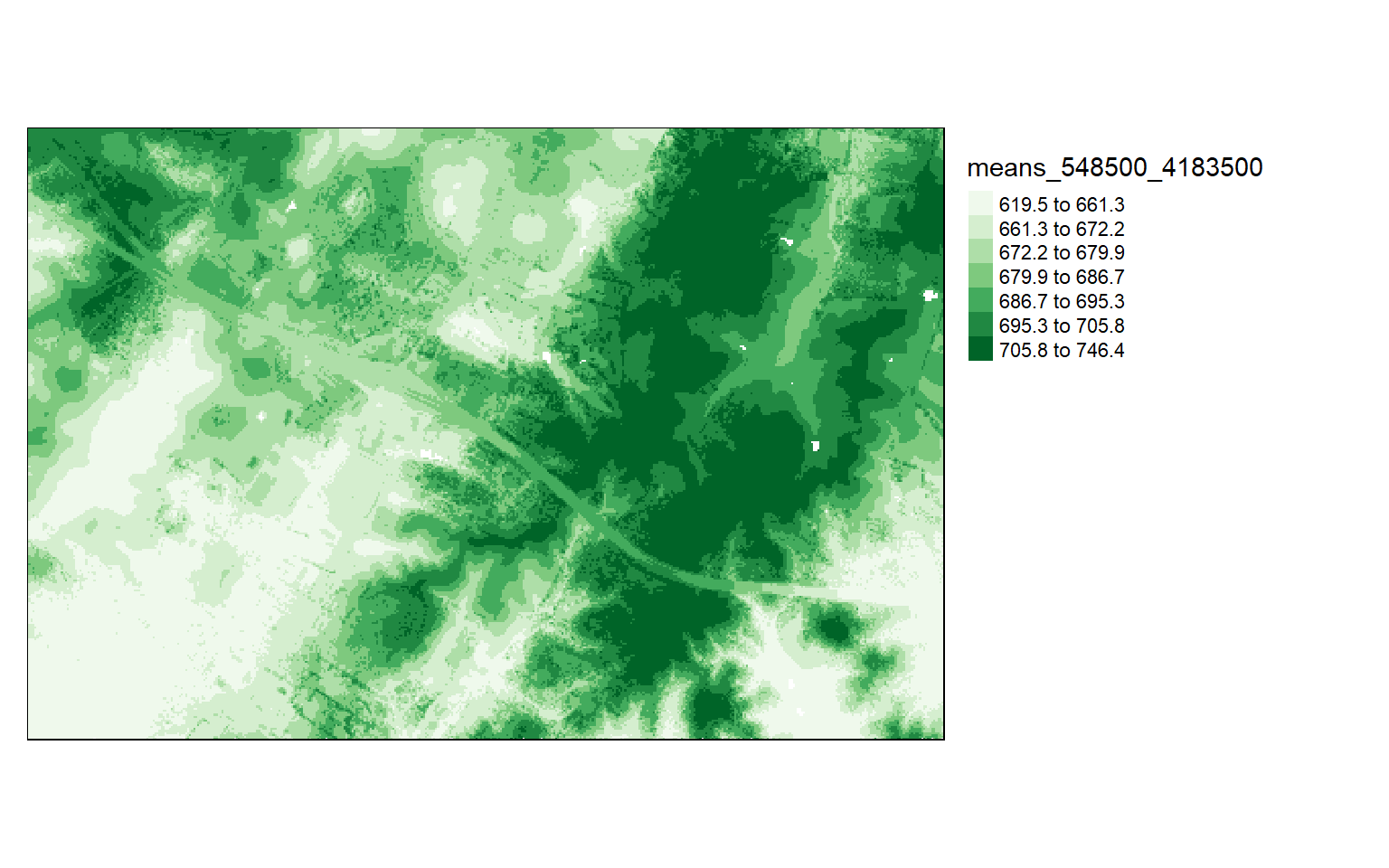
Visualize Return Intensity
Other than elevation measurements, LiDAR data can also store return intensity information. This is a measure of the proportion of the emitted energy that is associated with each return from each laser pulse. In the two code blocks below, I am visualizing the intensity values as the mean first return intensity within 5-by-5 meter cells.
This can provide an informative visualization of the LiDAR data.
opt_output_files(las_cat) <- "D:/ossa/las_out/int/int_{XLEFT}_{YBOTTOM}"
opt_filter(las_cat) <- "-keep_first"
int <- grid_metrics(las_cat, ~mean(Intensity), 5)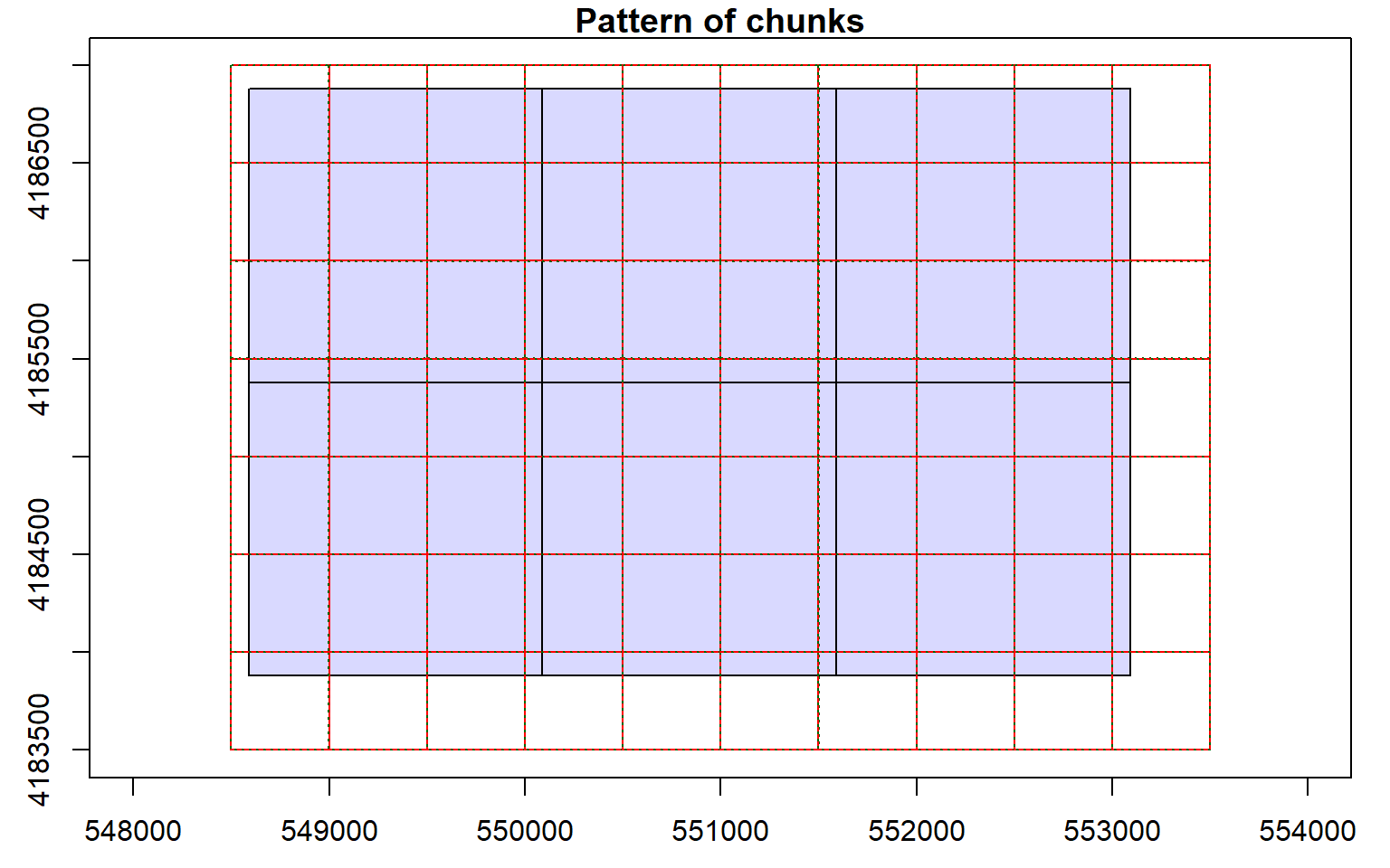
int[int<0]=0
tm_shape(int)+
tm_raster(style= "quantile", n=7, palette=get_brewer_pal("-Greys", n=7, plot=FALSE))+
tm_layout(legend.outside = TRUE)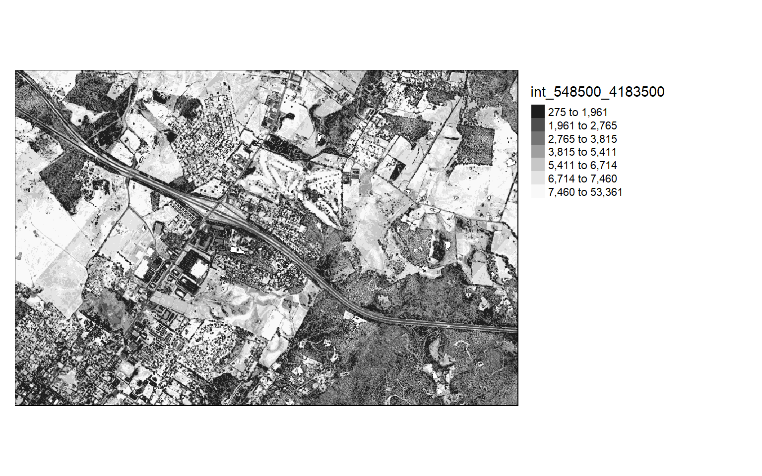
Voxelize Point Cloud Data
In this last example relating to LiDAR, I am reading in a single LAS file. I then generate a DTM from the point cloud then normalize the data using the DTM. Next, I generate voxels from the data. A voxel is a 3D raster where the smallest data unit is a 3D cube as opposed to a 2D grid cell. You can think of a voxel as a stack of cubes where each cube holds a measurement. In the example, I am generating a voxel in which each cube has dimensions of 5 meters in all three dimensions and stores the standard deviation of the normalized height measurements from the returns within it.
Voxels are used extensively when analyzing 3D point clouds. For example, they can be used to explore the 3D structure of forests.
las1 <- readLAS("D:/ossa/lidar/CO195.las")
las1_dtm <- grid_terrain(las1, res = 2, knnidw(k = 10, p = 2), keep_lowest = FALSE)
las1_n <- normalize_height(las1, las1_dtm)
las1_vox <- grid_metrics(las1_n, ~sd(Z), res = 5)
This is all we will cover here relating to the lidR package. However, there are many other valuable tools available. For example, there are methods for segmenting forest tree crowns and calculating metrics for each tree. If you work with LiDAR data, I recommend exploring this package further.
Image Processing
Normalized Difference Vegetation Index (NDVI)
Now we will explore methods for processing remotely sensed imagery. First, we will calculate the normalized difference vegetation index or NDVI from Landsat 8 Operational Land Imager (OLI) data.
First, I read in and visualize the data as a false-color composite. I am using the brick() function to read in the image since it is multi-band.
#You must set your own working directory.
ls8 <- brick("lidar/ls8example.tif")

plotRGB(ls8, r=5, g=4, b=3, stretch="lin")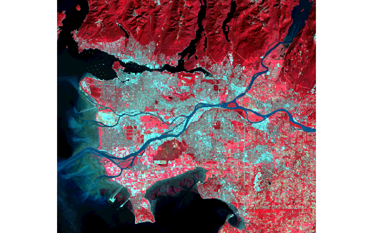
NDVI is calculated by differencing the NIR and red channels then dividing by the sum. Here, Band 5 is NIR and Band 4 is red. In the next code block I perform this calculation then plot the result with tmap.
Dark green areas indicate vegetated areas, such as forests and fields, while lighter areas indicate areas that are not vegetated or where the vegetation is unhealthy or stressed.
#You must set your own working directory.
ndvi <- (ls8$Layer_5-ls8$Layer_4)/((ls8$Layer_5+ls8$Layer_4)+.001)

tm_shape(ndvi)+
tm_raster(style= "quantile", n=7, palette=get_brewer_pal("Greens", n = 7, plot=FALSE))+
tm_layout(legend.outside = TRUE)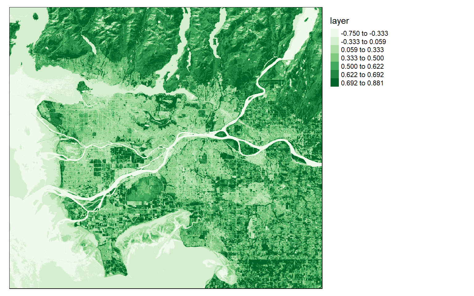
Principal Component Analysis (PCA)
You can generate principal component bands from a raw image using the rasterPCA() function from the RSToolbox() package. Principal component analysis (PCA) is used to generate new, uncorrelated data from correlated data. If we assume variability in data represents information then PCA is a useful means to capture the information content in fewer variables. When applied to imagery, we can generate uncorrelated bands from the raw imagery and potentially reduce the number of bands needed to represent the information.
In this example, I am applying PCA to all of the bands in the Landsat 8 image.
ls8_pca <- rasterPCA(ls8, nSamples = NULL, nComp = nlayers(ls8), spca = FALSE)The function generates a list object that contains the new image and information about the PCA analysis. I extract the resulting raster bands then displayed the first three principal components as a false-color image.
ls8_pca_img <- stack(ls8_pca$map)

plotRGB(ls8_pca_img, r=1, b=2, g=3, stretch="lin")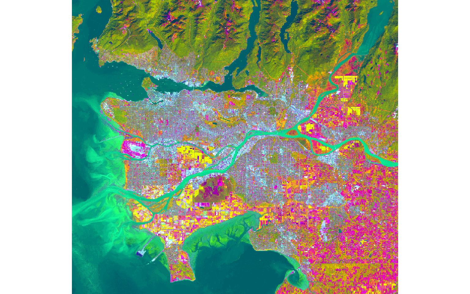
Now, I print the information about the PCA results. The majority of the variance is explained in the first three principle components.
ls8_pca$model
Call:
princomp(cor = spca, covmat = covMat[[1]])

Standard deviations:
    Comp.1     Comp.2     Comp.3     Comp.4     Comp.5     Comp.6     Comp.7
24.1772296 11.0168152  4.2179996  1.1382589  0.9980586  0.5632723  0.3406967

 7  variables and  3666706 observations.
Here are the Eigenvectors as an Eigen matrix. To obtain each PCA band, you would multiply the band values by the associated weights and add the results.
ls8_pca$model$loadings

Loadings:
        Comp.1 Comp.2 Comp.3 Comp.4 Comp.5 Comp.6 Comp.7
Layer_1         0.263  0.354  0.121  0.574  0.285  0.615
Layer_2         0.319  0.410  0.116  0.372        -0.758
Layer_3  0.104  0.287  0.390  0.124 -0.242 -0.796  0.215
Layer_4  0.126  0.392  0.325        -0.671  0.522
Layer_5  0.790 -0.529  0.290 -0.101
Layer_6  0.512  0.360 -0.544  0.559
Layer_7  0.285  0.429 -0.264 -0.795  0.150 -0.104

               Comp.1 Comp.2 Comp.3 Comp.4 Comp.5 Comp.6 Comp.7
SS loadings     1.000  1.000  1.000  1.000  1.000  1.000  1.000
Proportion Var  0.143  0.143  0.143  0.143  0.143  0.143  0.143
Cumulative Var  0.143  0.286  0.429  0.571  0.714  0.857  1.000
Tasseled Cap Tranformation
The tasseled cap transformation is similar to PCA; however, defined values are provided to generate brightness, greenness, and wetness bands from the original spectral bands. Different coefficients are used for different sensors, including Landsat Thematic Mapper (TM), Enhanced Thematic Mapper Plus (ETM+), and Operational Land Imager (OLI) data. In this example, I am calling in Landsat 7 ETM+ data using the brick() function.
The two images represent a portion of the Black Hills of South Dakota before and after a fire event.
pre <- brick("lidar/pre_ref.img")
post <- brick("lidar/post_ref.img")

plotRGB(pre, r=6, g=4, b=2, stretch="lin")
plotRGB(post, r=6, g=4, b=2, stretch="lin")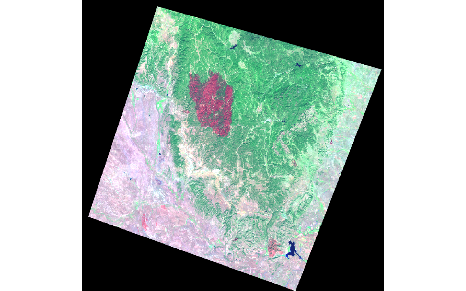
Once the data are read in, I rename the bands then apply the defined coefficients to each band for each transformation. I add the results to obtain the transformation.
In the next set of code, I stack the brightness, greenness, and wetness bands then display them as a false color composite. In the result, the extent of the fire is obvious.
names(pre) <- c("Blue", "Green", "Red", "NIR", "SWIR1", "SWIR2")
names(post) <- c("Blue", "Green", "Red", "NIR", "SWIR1", "SWIR2")

pre_brightness <- (pre$Blue*.3561) + (pre$Green*.3972) + (pre$Red*.3904) + (pre$NIR*.6966) + (pre$SWIR1*.2286) + (pre$SWIR2*.1596)
pre_greenness <- (pre$Blue*-.3344) + (pre$Green*-.3544) + (pre$Red*-.4556) + (pre$NIR*.6966) + (pre$SWIR1*-.0242) + (pre$SWIR2*-.2630)
pre_wetness <- (pre$Blue*.2626) + (pre$Green*.2141) + (pre$Red*.0926) + (pre$NIR*.0656) + (pre$SWIR1*-.7629) + (pre$SWIR2*-.5388)

post_brightness <- (post$Blue*.3561) + (post$Green*.3972) + (post$Red*.3904) + (post$NIR*.6966) + (post$SWIR1*.2286) + (post$SWIR2*.1596)
post_greenness <- (post$Blue*-.3344) + (post$Green*-.3544) + (post$Red*-.4556) + (post$NIR*.6966) + (post$SWIR1*-.0242) + (post$SWIR2*-.2630)
post_wetness <- (post$Blue*.2626) + (post$Green*.2141) + (post$Red*.0926) + (post$NIR*.0656) + (post$SWIR1*-.7629) + (post$SWIR2*-.5388)
pre_tc <- stack(pre_brightness, pre_greenness, pre_wetness)
post_tc <- stack(post_brightness, post_greenness, post_wetness)
plotRGB(pre_tc, r=3, g=2, b=1, stretch="lin")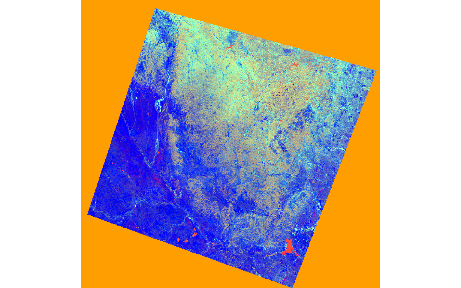
plotRGB(post_tc, r=3, g=2, b=1, stretch="lin")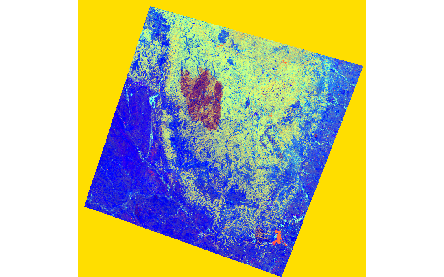
Differenced Normalized Burn Ratio (dNBR)
To explore the extent of the fire further, I will use the differenced normalized burn ratio (dNBR). This is obtained from the SWIR and NIR bands. A burned area will have a high SWIR reflectance and a low NIR reflectance in comparison to a forest extent. So, by calculating this index before and after a fire event, I can map the extent and severity of the fire. The code below shows this result. In the dNBR output, high values indicate burned areas.
pre_nbr <- (pre$NIR - pre$SWIR2)/((pre$NIR + pre$SWIR2)+.0001)

post_nbr <- (post$NIR - post$SWIR2)/((post$NIR + post$SWIR2)+.0001)

dnbr <- pre_nbr - post_nbr

dnbr[dnbr <= 0] <- NA

tm_shape(dnbr)+
tm_raster(style= "equal", n=7, palette=get_brewer_pal("YlOrRd", n = 7, plot=FALSE))+
tm_layout(legend.outside = TRUE)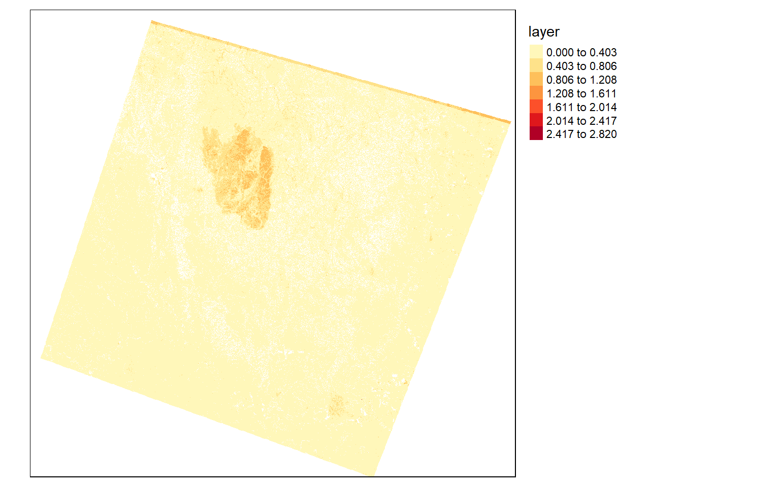
Moving Windows
It is common to analyze local patterns in image data by applying moving windows or kernels over the image to perform a transformation or summarization of the pixel values within the image. In R, this can be accomplished using the focal() function from the raster package.
In the first example, I am calculating the average NDVI value in 5-by-5 cell windows. This involves generating a kernel using the matrix() function. Specifically, I create a kernel with dimensions of 5-by-5 values, or a total of 25 cells. I then fill each cell with 1/25. Passing this over the grid will result in calculating the mean in each window.
ndvi5 <- focal(ndvi, w=matrix(1/25,nrow=5,ncol=5))

tm_shape(ndvi5)+
tm_raster(style= "quantile", n=7, palette=get_brewer_pal("Greens", n = 7, plot=FALSE))+
tm_layout(legend.outside = TRUE)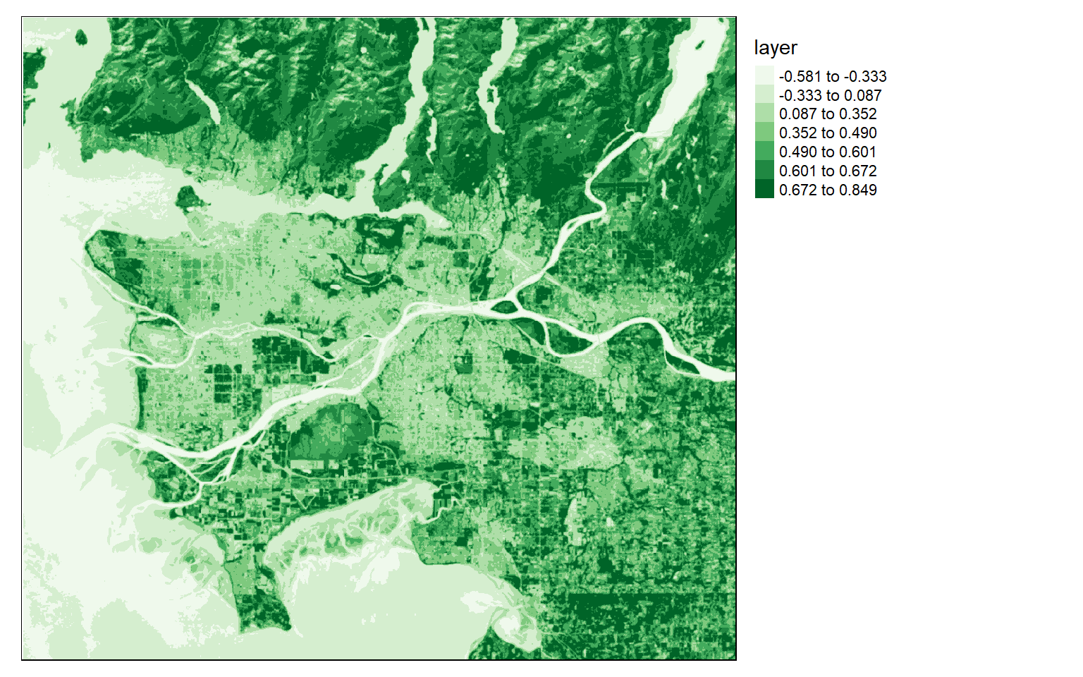
The Sobel filter is used to detect edges in images and raster data in general. It can be applied using different size kernels, such as 3-by-3 or 5-by-5. In the next code block, I am building then printing two 5-by-5 Sobel filters to detect edges in the x- and y-directions.
gx <- c(2, 2, 4, 2, 2, 1, 1, 2, 1, 1, 0, 0, 0, 0, 0, -1, -1, -2, -1, -1, -1, -2, -4, -2, -2)
gy <- c(2, 1, 0, -1, -2, 2, 1, 0, -1, -2, 4, 2, 0, -2, -4, 2, 1, 0, -1, -2, 2, 1, 0, -1, -2, 2, 1, 0, -1, -2)

gx_m <- matrix(gx, nrow=5, ncol=5, byrow=TRUE)
gx_m
     [,1] [,2] [,3] [,4] [,5]
[1,]    2    2    4    2    2
[2,]    1    1    2    1    1
[3,]    0    0    0    0    0
[4,]   -1   -1   -2   -1   -1
[5,]   -1   -2   -4   -2   -2
gy_m <- matrix(gy, nrow=5, ncol=5, byrow=TRUE)
gy_m
     [,1] [,2] [,3] [,4] [,5]
[1,]    2    1    0   -1   -2
[2,]    2    1    0   -1   -2
[3,]    4    2    0   -2   -4
[4,]    2    1    0   -1   -2
[5,]    2    1    0   -1   -2
Once the filters are generated, I apply them to the NDVI data to detect edges, or changes in NDVI values. Mapping the results, we can see that these filters do indeed highlight edges.
There are many different filters that can be applied to images. Fortunately, the process is effectively the same once you build the required filter as a matrix.
ndvi_edgex <- focal(ndvi, w=gx_m)
ndvi_edgey <- focal(ndvi, w=gy_m)

tm_shape(ndvi_edgex)+
tm_raster(style= "quantile", n=7, palette=get_brewer_pal("-Greys", n = 7, plot=FALSE))+
tm_layout(legend.outside = TRUE)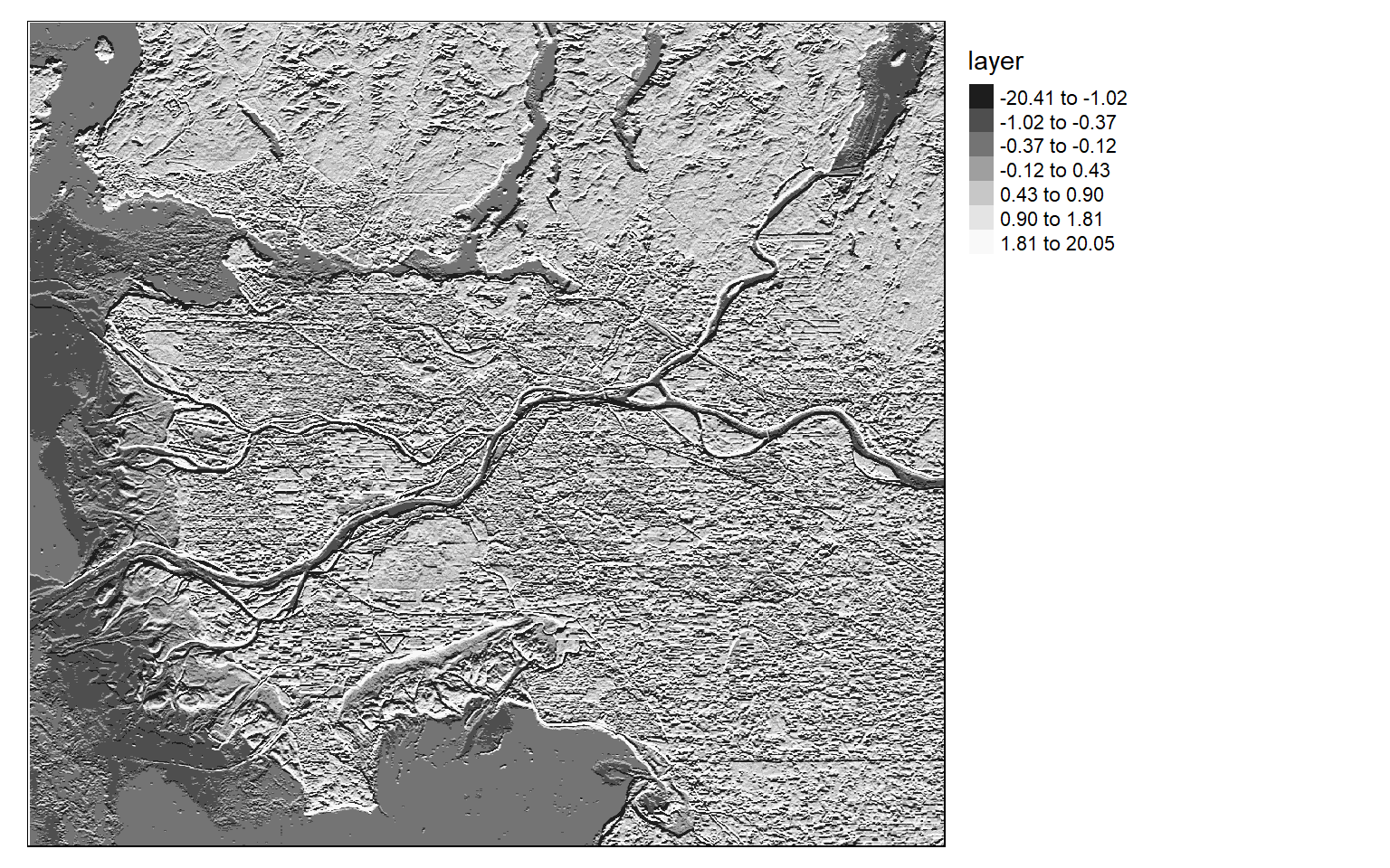
tm_shape(ndvi_edgey)+
tm_raster(style= "quantile", n=7, palette=get_brewer_pal("-Greys", n = 7, plot=FALSE))+
tm_layout(legend.outside = TRUE)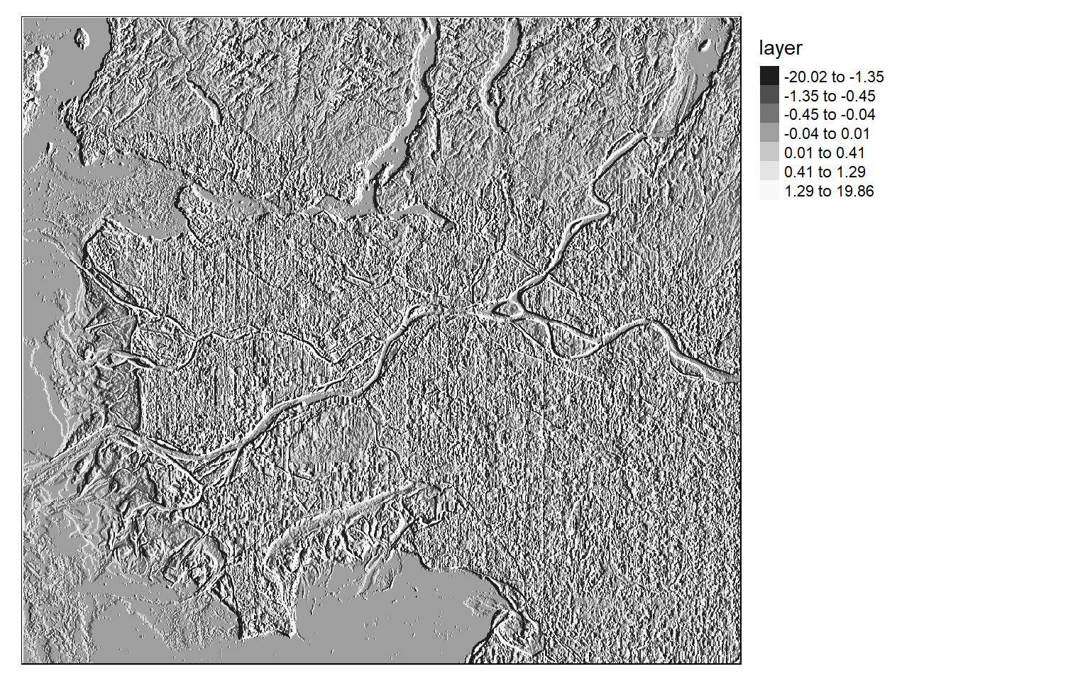
Concluding Remarks
The last two modules have provided a variety of examples for working with raster data and other remotely sensed data. If you would like to explore additional raster and image analysis techniques, have a look at the documentation for the raster and RStoolbox packages. You can also use terra to perform analyses on multispectral image data. Another common remote sensing task is to classify images into categories. We will cover this topic in later modules as an application of machine learning.